
RESUME - Project overview
Jump to: SOLUTION -Project implementation
Skills & Concepts demonstrated
A reporter writes an article about 40-year movie industry for MovieMaker Magazine. Dataset containing IMDb movie details was downloaded from The kaggle website. The task of the assigned Data Analyst is to organize data, analyze it and to produce actionable insights to the customer as a basis for writing an article.
Problem Statement
The Dataset contains details on movies released in the period 1980-2020. The format of the Dataset is CSV file, and since the customer is reporter writing an article it is not very useful for them to get some useful insights from raw CSV file.
Skills & Concepts demonstrated
There are following Python features used in this project
Customer wants to answer the following questions:
Questions
1-Categorize movie Score using the following key, based on the range from lowest to highest movie score: Excellent (top 25%), Very good(65-75%), Good(55-65%), Average(45-55%), Poor(below 45%).
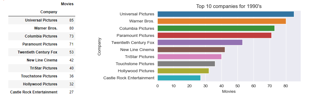
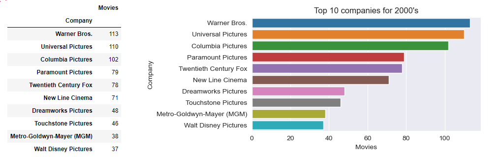
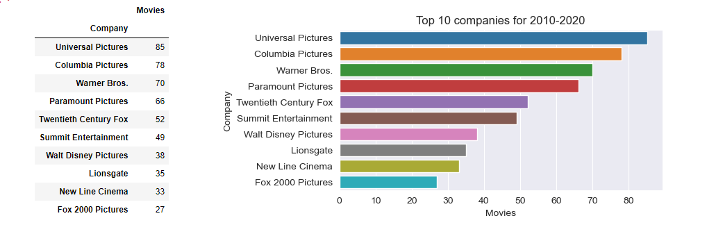
2-Find top 10 companies by number of movies made for each decade and top 5 companies overall.
3-Get top 10 highest rated movies and visualize insights showing director in legend. Find top 10 most productive directors overall (by movies directed).
4-Find overall correlation between movie score and the total nett profit. Nett profit is the difference between gross revenue and budget.
5-Find correlation between movie score and return of investment (ROI) for each decade. ROI is the ratio between the nett profit and budget.
Insights
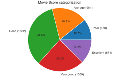
1. There the most movies (1,862) in Good category (34.5%), followed by Very good (1,309) movies (24.2%). The 3rd place (981) belongs to Average movies (18.2%), followed by Excellent (671) movies (12.4%) and the Poor (578) movie category (10.7%)
2. The top company overall by movies made is Universal Pictures (330), followed by Columbia Pictures (301), Warner Bros. (298), Paramount Pictures (278) and Twentieth Century Fox (209)


3. The highest rated (9.3) movie is The Shawshank Redemption, followed by The Dark Knight (9.0). The Lord of the Rings: The Return of The King (8.9), Pulp Fiction (8.9) and Schindler's List (8.9) share the 3rd, the 4th and the 5th place. The places from 6 to 9 are shared by Inception (8.8), Fight Club (8.8), The Lord of The Rings: The Fellowship of the Ring (8.8) and Forrest Gump (8.8). In the 10th place is the movie Star Wars: Episode V - The Empire Strikes Back (8.7)


4. The correlation is positive and small (0.24). After removing high and low outliers (5% in total) from the Profit variable, the correlation factor is even decreased (0.20) so it remained in the category of small correlation
5. For each decade the correlation is positive and negligible (0.09) before removing outliers. After removing 3% high outliers from ROI variable, the correlation factor increased signifficantly (0.26) nevertheless it remained small.
SOLUTION - Project implementation
Back to: RESUME -Project overview
The raw Data source is CSV file:
From the
GitHub repository
it can be downloaded
Before processing business questions, the data will be gathered from CSV file and assessed. Based on assessments outcome data will be cleaned and transfomered i.e. data types will be converted to appropriate types depending on values containing.
0.1-Gathering Data
Dataset is a single CSV file that will be imported using pandas, into a DataFrame object. DataFrame is 2-dimensional structure that stores data in rows and columns, a.k.a. Series. The first step is importing Python libraries that will be used - pandas, matplotlib and seaborn. The Dataset is loaded directly from GitHub repository into pandas DataFrame.
import pandas as pd
import seaborn as sns
import matplotlib.pyplot as plt
df=pd.read_csv("https://github.com/berislav-vidakovic/Portfolio/blob/main/IMDbMovies/ImdbMovies.csv?raw=true")
pd.options.display.max_rows = 5 #limit row count to display
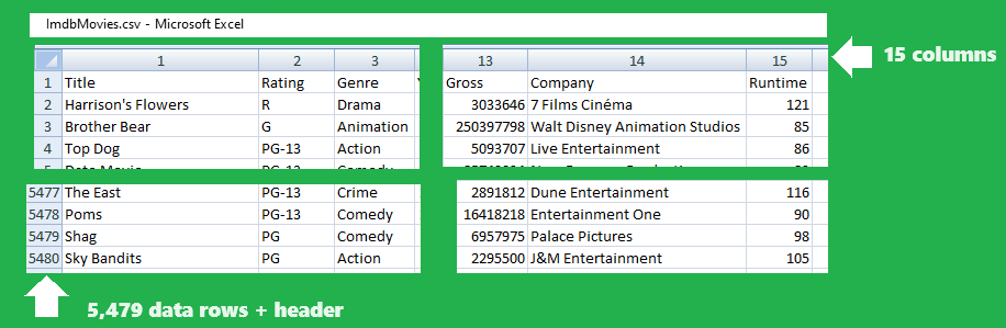
df # show DataFrame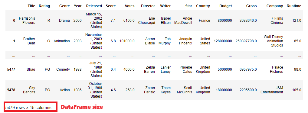
There are shown first and last 2 rows (by default there would be 5+5 rows, that can be controlled by changing max_rows display option. Below the table there are some basic dataset information - row and column count. However, there are much more information about data (such as column data types, NULL/non-NULL value count etc.) that can be obtained using different pandas methods and attributes of DataFrame and Series classes.
0.2-Assessing Data
In this section data will be explored in general, such as showing few first and last rows, column data types, max/min/mean values per column, detecting null values and duplicates.
Using head() and tail() method on DataFrame and passing number of rows it will be shown first and last n rows. By default, if no paramater passed, the first/last 5 rows are returned. Pretty formatting of floats - 2 decimals and thousand separator - is accomplished by changing the float_format display option and passing in a lambda function
pd.set_option('display.float_format', lambda x: '{:,.2f}'.format(x)) # format float as 1,000.00
df.head(3)
df.tail(3)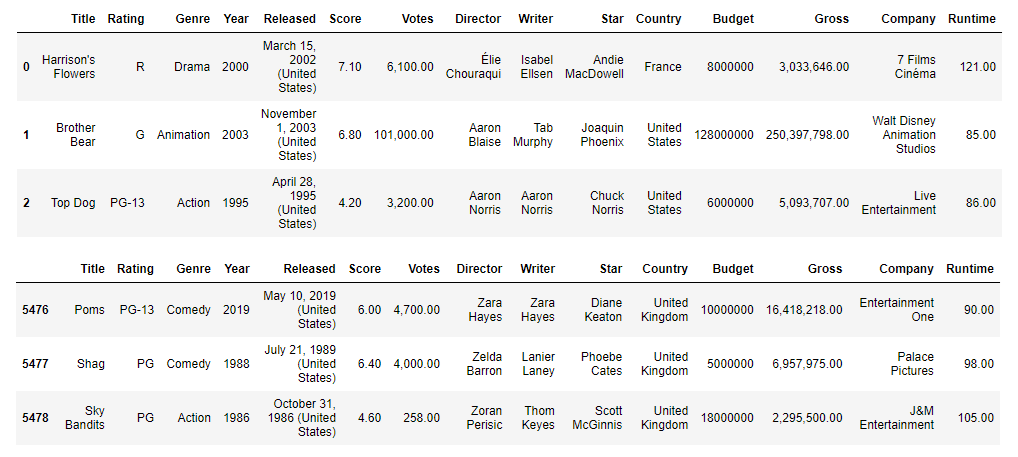
Using attribute shape on DataFrame object there will be shown row and column count as tuple data type. It can formatted as well, with accessing each tuple member separately in order to enable more user-friendly information. Using info() method on DataFrame object there will be shown column data types and more details about DataFrame.
df.shape
print("Rows: ", df.shape[0], "Columns:", df.shape[1])
df.info()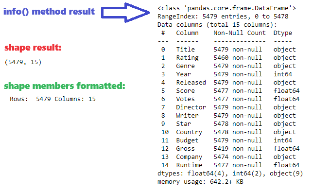
Result of info() method already provide insight on null-values for some columns, since there is lower non-null value count than total row count. Null values will be later investigated and visualized.
The next method is describe() that generates descriptive statistics. Descriptive statistics include those that summarize the central tendency, dispersion and shape of a dataset’s distribution, excluding NaN values.
pd.set_option('display.float_format', lambda x: '{:,.2f}'.format(x)) # format float as 1,000.00
currentSetting = pd.options.display.max_rows
pd.options.display.max_rows = 15 # needed for describe() method only, transparently changed
df.describe()
df.describe(include='all')
pd.options.display.max_rows = currentSetting # reset to previous value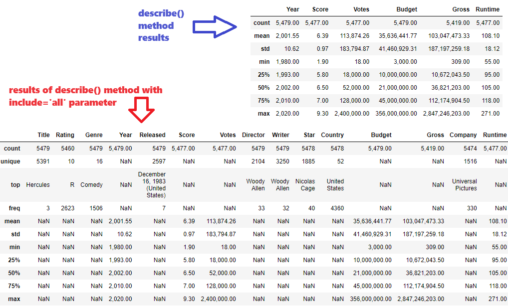
Checking duplicates starts with examining are there any using method any(), if there are their count is checked using function sum() and duplicate rows are shown using boolean indexing for filtering. These information will be used in Data cleaning section, where duplicates will be removed.
df.duplicated().any() #Check if there are duplicates at all
df.duplicated().sum() #How many duplicate rows are there
df[df.duplicated()==True] #Show duplicate rows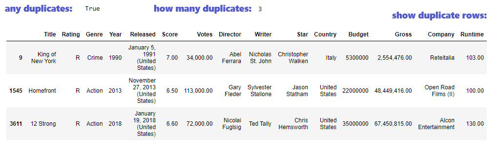
Check missing values (or NaN values, or null values) will start with extracting columns containing any null values. After that there is shown for those column missing value count and percentage. Results are visualized in seaborn heatmap.
dfMissing = df.isnull()  #bool for each value - True for missing value
colsMissing = dfMissing.any() #are there any missing values
colsMissing #show if there are for each column

countMissing=df[df.columns[colsMissing]].isnull().sum() #show only columns with missing values
countMissing #show missing value count
countMissing * 100 / len(df) #show missing value percentage

ax=sns.heatmap(dfMissing) #visualize missing values with seaborn heatmap
ax.invert_yaxis() #show values on y-axis in bottom-up direction
plt.title('Missing values')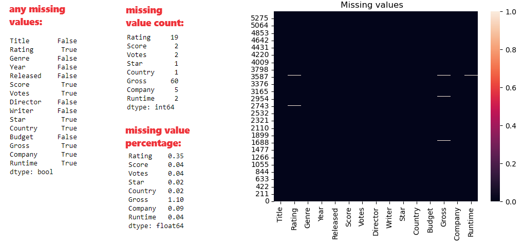
0.3-Data cleaning
Within data cleaning process there will be removed duplicate and missing values, using information obtained in previous section of Data assessment to control the process. After dropping dupes and missing values, DataFrame will be re-indexed. Removing duplicates will be the first step, using drop_duplicates() method on DataFrame object.
df.shape # check data shape before starting cleaning
df.drop_duplicates(inplace=True) #removing duplicates
df.duplicated().any() #double check for dupes after dropping
df.shape # duplicates removed, lower row count
Removing rows that contain any missing value will be done using dropna() method on DataFrame object.
df.info() # check for missing value count before dropping them
df.dropna(inplace=True)
df.info() # check for missing value count after dropping them
df.isnull().any() # double check if there are any more missing values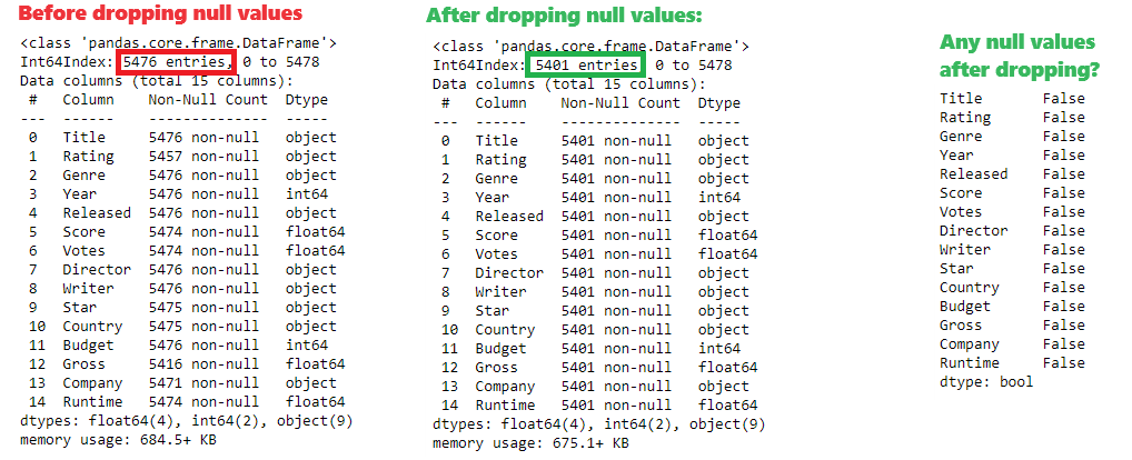
After deleting NULLs and duplicates, it is recommended to reset index. By setting drop=True, the current index column will be removed, while inplace=True ensures the changes are applied directly to the DataFrame without creating a new one.
df.reset_index(inplace=True, drop=True)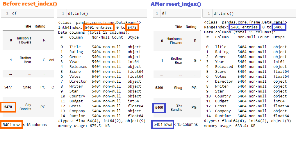
0.4-Data transformation
Depending on the range of values stored, value type and common sense, there will be assessed current column data types and determined optimal data type for each particular column.
Datetime Series conversion
Although there are 2 columns with date -[Year] and [Released] - neither of them has datetime data type. We need 1 column of datetime data type as the single source of truth for movie date. The column [Released] is considered to contain relevant date information, nevertheless the column [Year] would be easier to convert to datetime type. To be on the safe side it has to be checked the data consistency between the 2 columns, and before comparison both columns have to be converted to datetime type. In order to convert integer [Year] column to datetime it has to be specified format, otherwise the conversion will not work properly.
df.insert(4,'YearDt','') #insert helper column for conversion testing

df['YearDt']=pd.to_datetime(df['Year']) #conversion with no format specified
df[['Year','YearDt']] #bad outcome

df['YearDt']=pd.to_datetime(df['Year'], format='%Y') #conversion with format specified
df[['Year','YearDt']] #good outcome

df.drop(columns='Year', inplace=True) #remove original integer column
df.rename(columns={'YearDt': 'Year' }, inplace=True) #rename helper column
df #show actual DataFrame
df.info() #check data types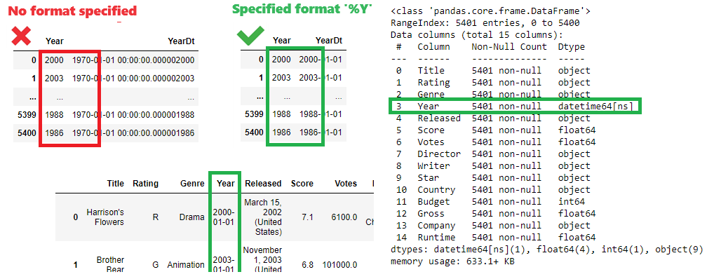
Conversion of [Released] column to datetime type cannot be accomplished directly since there is also state name in that column. First the column has to be split using parenthesis separator, to extract string portion that is clean date. After that column can be converted to datetime type. Argument expand=True in split() function means that result will be written as a DataFrame with one column for each substring, otherwise (with expand=False) all substrings will be within single Series object as items in the list. After splitting it can be compared year in both columns, to check data consistency.
df[['Released']] #original column
dfSplit=df['Released'].str.split('(', expand=False) #split items to list in one Series
dfSplit=df['Released'].str.split('(', expand=True) #split items to more Series in DataFrame
df.insert(5,'ReleasedDt','') #insert helper column for conversion testing
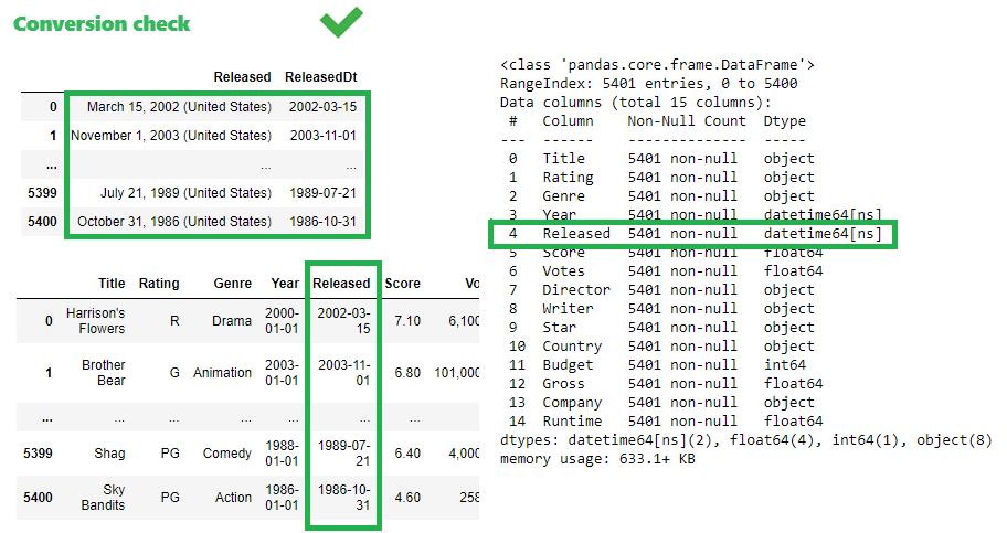
df['ReleasedDt']=pd.to_datetime(dfSplit[0]) #conversion the date part to helper column
df[['Released','ReleasedDt']] #check if conversion was successful
df.drop(columns='Released', inplace=True) #remove original column
df.rename(columns={'ReleasedDt': 'Released' }, inplace=True) #rename helper column
df #show actual DataFrame
df.info() #check data types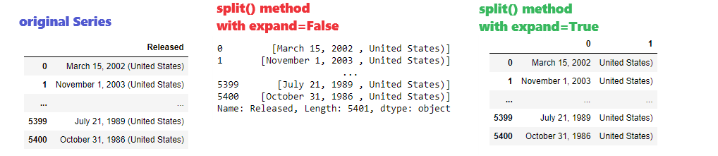
After applying split method with parameter expand=True the conversion is done with first Series from new DataFrame dfSplit, and results are acceptable:
The next step is data consistency check. i.e. extract the year of dates in both columns and compare them
df[df['Year'].dt.year != df['Released'].dt.year] #select rows with incosistent data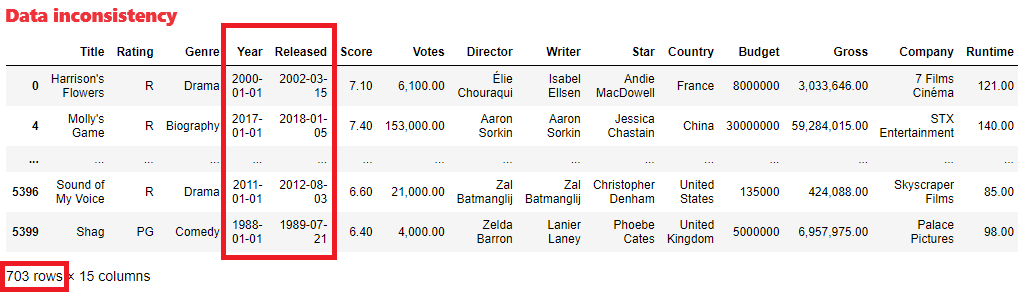
There are 703 rows with inconsistent dates. The [Release] column contains complete date including month and day, so [Year] column will be dropped and the single source of truth for movie date will remain in the [Released] column.
df.drop(columns='Year', inplace=True)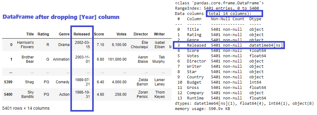
String Series conversion
There are columns containing string data but data type is object after data imported. Those columns will be converted to string data type.
lsStringColumns =['Title', 'Rating', 'Genre', 'Director', 'Writer', 'Star', 'Country', 'Company'] #string column list
df[lsStringColumns] #show string columns before conversion

for col in lsStringColumns:
    df[col] = df[col].astype('string') #convert each column to string type

df[lsStringColumns] #show string columns after conversion
df.info() #check data types after conversion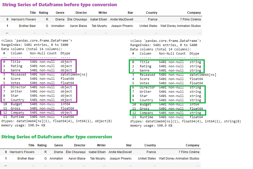
Numerical Series conversion
There are few numerical columns that will be converted to proper data type depending on value range and kind of information they keep. Using aggregate functions min and max there is a range shown for each numerical column
lsNumColumns =['Score', 'Votes', 'Budget', 'Gross', 'Runtime'] #numerical column list
dfNum = df[lsNumColumns].copy() # get numerical columns only
pd.set_option('display.float_format', lambda x: '{:,.2f}'.format(x)) # format float as 1,000.00
dfNum['Budget']=dfNum['Budget'].apply(lambda x: '{:,}'.format(x)) # format integer as 1,000
dfNum # show numerical columns

dfRange=df[lsNumColumns].agg(['min','max']) # get value range for each numerical column
dfRange['Budget']=dfRange['Budget'].apply(lambda x: '{:,}'.format(x)) # format integer as 1,000
dfRange # show column ranges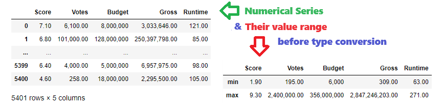
Taking data statistics into account, the following types would be the best fit for each column:
df['Score'] = df['Score'].astype('float16')
df['Votes'] = df['Votes'].astype('int32')
df['Budget'] = df['Budget'].astype('int32')
df['Gross'] = df['Gross'].astype('int64')
df['Runtime'] = df['Runtime'].astype('int16')
df.info()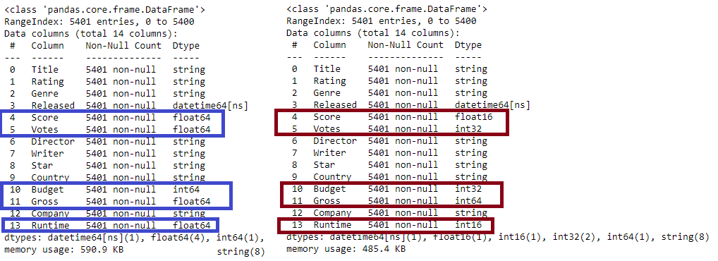
Double check values and ranges after data type conversion:
dfNum = df[lsNumColumns].copy() #get numeric columns only
dfNum['Budget']=dfNum['Budget'].apply(lambda x: '{:,}'.format(x)) #format integer as 1,000
dfNum # show numerical columns

dfRange=df[lsNumColumns].agg(['min','max']) #get value range for each numerical column
dfRange['Budget']=dfRange['Budget'].apply(lambda x: '{:,}'.format(x)) #format integer as 1,000
dfRange['Votes']=dfRange['Votes'].apply(lambda x: '{:,}'.format(x)) #format integer as 1,000
dfRange['Gross']=dfRange['Gross'].apply(lambda x: '{:,}'.format(x)) #format integer as 1,000
dfRange #show column ranges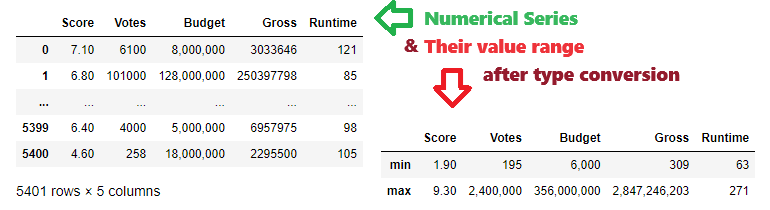
1-Data binning - movie score categorization
The first step in binning of Series 'Score' will be to check the value range and define the expected results i.e. threshold for the particular score category. Let's look at column statistic data:
df['Score'].agg(['min','max', 'mean']) # get some statistics for Score column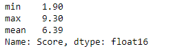
Distribution of Score column values can be visualized as follows:
def PlotNumDistribution(seriesName, title):
    plt.figure(figsize=(10,4))
    plt.title(title)
    sns.set_style('darkgrid')
    df[seriesName].plot(kind='hist')
    plt.xlabel(seriesName)

PlotNumDistribution('Score','Score distribution')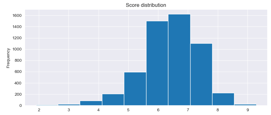
As required binning is defined with percentage, it is neccessary to calculate the actual values that will be used for binning criterium, the lower and upper limits for category intervals.
pd.set_option('display.float_format', lambda x: '{:,.2f}'.format(x)) # format float as 1,000.00
binLabels=['Poor', 'Average', 'Good', 'Very good', 'Excellent']
binLimits=[0.45, 0.55, 0.65, 0.75]

# extending bin limits to start with 0 and end with 1
def ExtendLimits(lsLimits):
    lsExtended =[0]
    lsExtended.extend(lsLimits)
    lsExtended.extend([1])
    return lsExtended

# mapping bin limits to actual values in numerical Series
def MapLimits(lsLimits, low, high):
    lsExt = ExtendLimits(lsLimits) #add 0 to beginning and 1 to end
    lsMapped =[]
    lenList = len(lsExt) # limit list length
    diff=high-low
    for i in range(lenList):
        limit11 = low + lsExt[i] * diff
        lsMapped.append(limit11)
    return lsMapped

#function fills dictionary with label as key and range tuple as value
def CalcLimits(dict1, binLab, binLim, SeriesNum):
    # get range from Datafrane numerical Series passed
    low = df[SeriesNum].min()
    high = df[SeriesNum].max()
    # mapping bin limits to actual data
    binLimLocal = MapLimits(binLim, low, high)
    lenList = len(binLab) # label list length
    for i in range(lenList):
        low1 = binLimLocal[i]
        high1 = binLimLocal[i+1]
        dict1[binLab[i]] = (low1, high1) # dict key is label, value is tuple(low,high)
    return

# Formatting string from passed dict (label as key, range tuple as value)
def FormatDict(dict1):
    str=''
    for key, value in dict1.items():
        str += key + ': '
        str += '-'.join(format(f, '.2f') for f in value)
        str += '\n'
    return str

# Calculate limit for each category interval
dictLimits = {}
CalcLimits(dictLimits, binLabels, binLimits, 'Score')

# Print required categorization
strRanges = FormatDict(dictLimits)
print('Required binning of Score Series to categories:')
print(strRanges)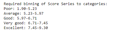
Now it's clearly defined which are exactly the intervals for each particular category. The first try will be using qcut method, as there are percentages defined that can be passed to it (using function for extending the initial list of limits with leading 0 and trailing 1)
# The easiest way would be using qcut
lsLimits = ExtendLimits(binLimits) #adding leading 0 and trailing 1 to the list
df['ScoreCat']=pd.qcut(df['Score'], lsLimits, labels=binLabels)

# Let's see the results
#function fills dictionary from DataFrame with Category as key and range tuple as value
def GetCategoryRange(dict1, SeriesCat, SeriesNum):
    for label in binLabels:
        low=df[df[SeriesCat] == label][SeriesNum].min()
        high=df[df[SeriesCat] == label][SeriesNum].max()
        dict1[label] = (low, high)
    return

dict1={}
GetCategoryRange(dict1, 'ScoreCat', 'Score')
# Print accomplished categorization
strRanges = FormatDict(dict1)
print('Using qcut - Accomplished binning of Score Series to categories:')
print(strRanges) # bad outcome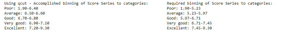
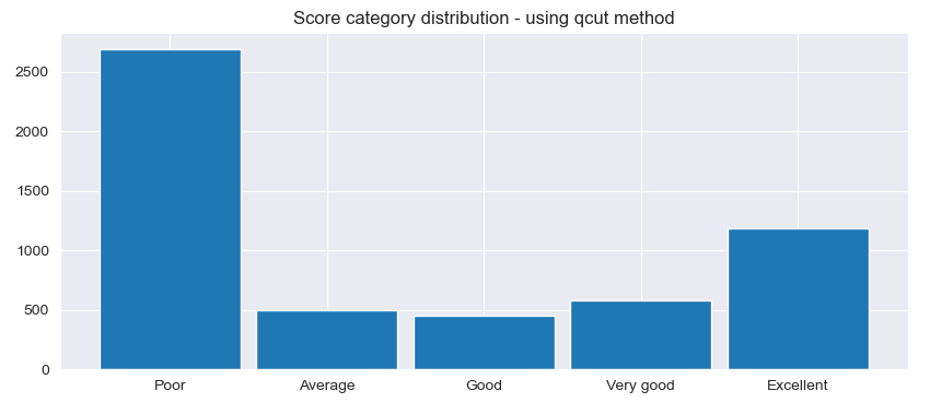
It seems that results are not as expected. The pandas documentation describes qcut as a “Quantile-based discretization function.” This basically means that qcut tries to divide up the underlying data into equal sized bins. The function defines the bins using percentiles based on the distribution of the data, not the actual numeric edges of the bins. Distribution of new category column can be visualized
# Show category distribution
def PlotCatDistribution(seriesName, orderX, title):
    plt.figure(figsize=(10,4))
    plt.title(title)
    df[seriesName].value_counts().loc[orderX].plot.bar(width=0.9) #using loc to define x-axis order
    plt.xticks(rotation=0)

PlotCatDistribution('ScoreCat', binLabels, 'Score category distribution - using qcut method')
Finally, expected categorization will be accomplished using cut method.
# The better choice will be using cut method
low=df['Score'].min()
high=df['Score'].max()
lsLimits= MapLimits(binLimits,low,high) # extending and mapping limits to actual values
df['ScoreCat']=pd.cut(df['Score'], lsLimits, labels=binLabels, include_lowest=True)

# Let' see the results
dict1 ={}
GetCategoryRange(dict1, 'ScoreCat', 'Score')
# Print accomplished categorization
strRanges = FormatDict(dict1)
print('Using cut - Accomplished binning of Score Series to categories:')
print(strRanges) #good outcome
# Plot accomplished categorization
PlotCatDistribution('ScoreCat', binLabels, 'Score category distribution - using cut method')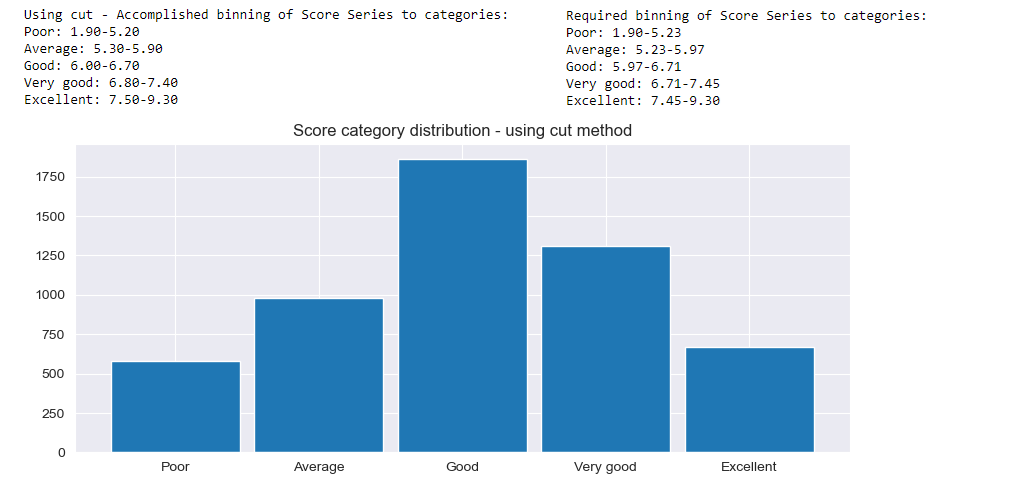
Nevertheless, comparing to required binning limits, it seems there are some gaps. This is probably because there are no Score values that fall within those intervals. To be on the safe side it can easily be checked:
df['Score'].between(5.2,5.3, inclusive='neither').any() or df['Score'].between(5.9,6.0, inclusive='neither').any() or \
df['Score'].between(6.7,6.8, inclusive='neither').any() or df['Score'].between(7.4,7.5, inclusive='neither').any()
The final categorization of Score column visualized in pie chart:
def PlotPieChart(seriesValues, lsBinLabels, sTitle):
      nCatCount=[]
      for label in lsBinLabels:
          nCatCount.append(len(df[df[seriesValues] == label]))

      lsLabels = []
      lenList = len(lsBinLabels)
      for i in range(lenList):
          lsLabels.append(lsBinLabels[i] + '(' + str(nCatCount[i]) + ')')

      fig, ax = plt.subplots()
      ax.pie(nCatCount, labels=lsLabels, autopct='%1.1f%%')
      plt.title(sTitle)

PlotPieChart('ScoreCat', binLabels, 'Movie Score categorization' )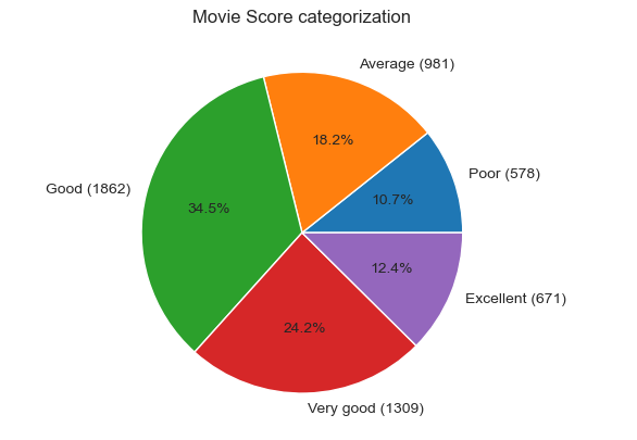
2-Feature engineering - extending data model with decade, ROI and Profit
Get top 10 companies by number of movies made, overall and for each decade.
In order to meet requirements of next business questions there should be created 3 new column: Decade, ROI and Profit. To create Decade category, bins passed to cut method have to the same type as the base column - it is [Released] column od the type datetime:
binLabelsD=["1980's", "1990's","2000's", "2010-2020"]
binsD=[1980, 1990, 2000, 2010, 2021]
# Convert bins to be datetime type such as column that is binned
binsDt =[]
for bin in binsD:
    binsDt.append(pd.to_datetime(bin, format='%Y'))
df['Decade']=pd.cut(df['Released'], bins=binsDt, labels=binLabelsD)
# Call wrapper function to plot the pie chart
PlotPieChart('Decade', binLabelsD, 'Released year categorized by decade' )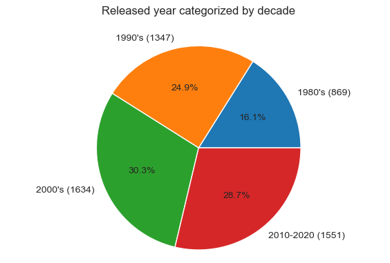
There are 2 more columns created and checked in a formatted view
df['Profit']=df['Gross']-df['Budget']
df['ROI']=(df['Gross']-df['Budget'])/df['Budget']

def FormatIntegerSeries(df1, seriesName):
    df1[seriesName]=df1[seriesName].apply(lambda x: '{:,}'.format(x)) #format integer as 1,000
pd.set_option('display.float_format', lambda x: '{:,.2f}'.format(x)) # format float as 1,000.00

dfFormatted = df[['Title', 'Released', 'Decade', 'Budget', 'Gross', 'Profit', 'ROI']].copy()
FormatIntegerSeries(dfFormatted, 'Budget')
FormatIntegerSeries(dfFormatted, 'Gross')
FormatIntegerSeries(dfFormatted, 'Profit')
dfFormatted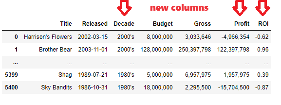
The business question of top 10 companies per decade will be answered using value_counts() and barplot, as well as the question for top 5 companies overall
def GetTopCompaniesForDecade(sDecade):
    dfDecade = df[df['Decade'] == sDecade] # filter by Decade passed
    seriesValueCounts =dfDecade['Company'].value_counts().head(10) # get top 10 of value_counts()
    dict1 = {'Company': seriesValueCounts.keys(), 'Movies': seriesValueCounts}
    df2=pd.DataFrame(dict1)
    df2=df2.set_index('Company')
    return df2

def ShowTopCompaniesForDecade(dframe,sDecade):
    plt.figure(figsize=(6,3))
    sns.barplot(x='Movies', y=dframe.index, data=dframe)
    plt.title('Top 10 companies for ' + sDecade)
    return

for decade in binLabelsD: # For each Decade prepare data and plot
    df2 = GetTopCompaniesForDecade(decade)
ShowTopCompaniesForDecade( df2, decade) 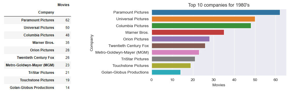
Top 5 companies overall will be found the same way but without Decade filter:
seriesValueCounts =df['Company'].value_counts().head(5) # get top 5 of value_counts()
dict1 = {'Company': seriesValueCounts.keys(), 'Movies': seriesValueCounts}
df2=pd.DataFrame(dict1)
df2=df2.set_index('Company')
plt.figure(figsize=(6,3))
sns.barplot(x='Movies', y=df2.index, data=df2)
plt.title('Top 5 companies 1980-2020')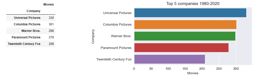
3-Univariate analysis - movie Runtime and Votes Analysis & Removing Outliers
Get top 10 highest rated movies and visualize insights showing director in legend. For each of the top 3 genres overall, find top 5 movies by movie score.
Movie [Runtime] distribution shows the central tendancy to 90-100 minute movie.
PlotNumDistribution(df, 'Runtime','Runtime column distribution')
df[['Runtime']].describe()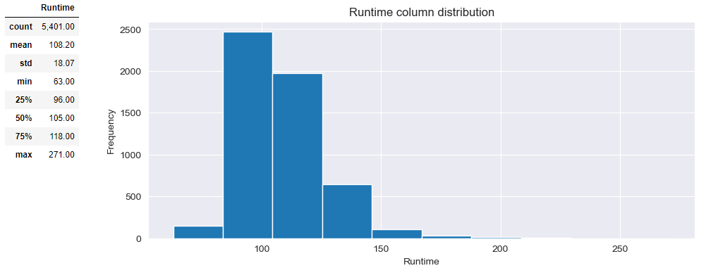
Removing outliers will enable more detailed insight. First let's check the outlier count/percentage
#check how many outliers are there with Runtime lower than 84 and higher than 150 minutes
nOutliersH = len(df[df['Runtime'] > 150])
nPercentH = nOutliersH / len(df) * 100
nOutliersL = len(df[df['Runtime'] < 84])
nPercentL = nOutliersL / len(df) * 100
print("Outliers with Runtime < 84 minutes: {:.0f} ({:.2f}%)\n\
Outliers with Runtime > 150 minutes: {:.0f} ({:.2f}%)".format(nOutliersL,nPercentL,nOutliersH,nPercentH))
Since in total there are 5% they can be removed without signifficant affecting the data quality
# Remove outliers
df2 = df[df['Runtime'].between(84,150)]
PlotNumDistribution(df2, 'Runtime','Runtime column distribution (removed outliers)')
df2[['Runtime']].describe()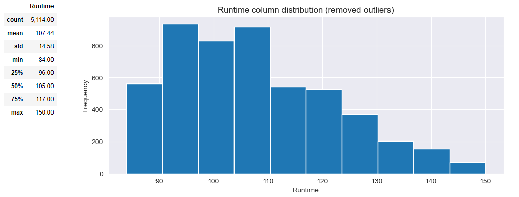
Distribution of [Votes] shows the central tendancy to around 50,000, but since there are outliers with much higher values it's difficult to tell before removing outliers.
PlotNumDistribution(df, 'Votes','Votes column distribution')
df[['Votes']].describe()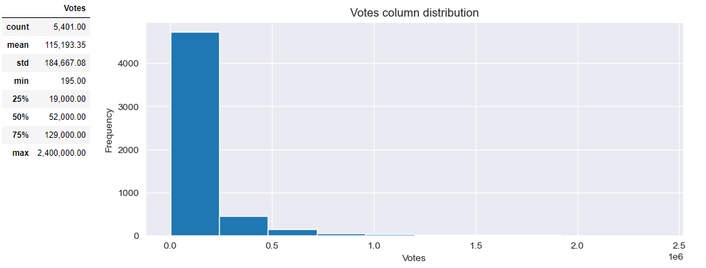
Removing outliers will enable more detailed insight. First let's check the outlier count/percentage
# Check how many  outliers over 450000
nOutliersH = len(df[df['Votes'] > 450000])
nPercentH = nOutliersH / len(df) * 100
print("Outliers with Votes > 450000 {:.0f} ({:.2f}%)".format(nOutliersH,nPercentH))
Since in total there are almost 5% they can be removed using quantile method, passing the percentage of values we want to keep (95% in this case) without signifficant affecting the data quality. After outliers removed, central tendancy can be better estimated, it is around 20,000
# Remove outliers for better distribution insight
q=df['Votes'].quantile(0.95)
df95=df[df['Votes'] < q]
PlotNumDistribution(df95, 'Votes','Votes column distribution (removed outliers)')
df95[['Votes']].describe()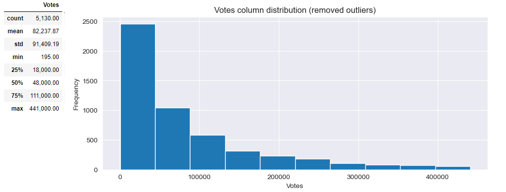
There is business question to answer about top movies and directors.
colsToShow =['Title','Score','Director','Released','Writer','Company', 'Votes', 'Runtime']
top10_rated=df.nlargest(10,'Score')[colsToShow].set_index('Title')
top10_rated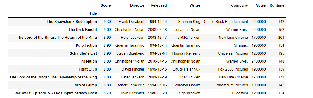
Finally results are visualized:
sns.barplot(x='Score', y=top10_rated.index, data=top10_rated,hue='Director', dodge=False)
sns.set_style('darkgrid')
plt.title('Top 10 highest rated movies')
plt.legend(bbox_to_anchor=(1.05,1),loc=2)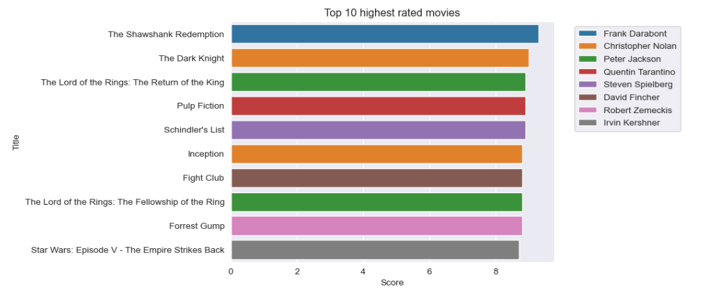
The most productive directors overall:
seriesValueCounts=df.groupby('Director')['Title'].count().sort_values(ascending=False).head(10)
dict1 = {'Director': seriesValueCounts.keys(), 'Movies made': seriesValueCounts}
df2=pd.DataFrame(dict1)
df2=df2.set_index('Director')
#prepare data for bar plot
Dirs = list(seriesValueCounts.keys())
Titles = list(seriesValueCounts)
fig = plt.figure(figsize = (9.5, 4))
# creating the bar plot
plt.bar(Dirs, Titles, color ='darkgreen', width = 0.8)
plt.xlabel("Director")
plt.ylabel("Movies made 1980-2020")
plt.title("Top 10 the most productive Directors")
plt.xticks(rotation=45)
plt.show()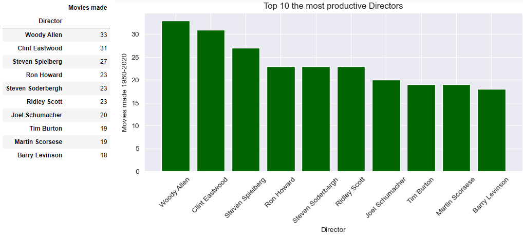
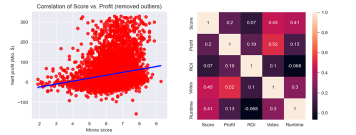
4-Bivariate analysis - correlation of Score vs. Profit
Find overall correlation between movie score and the total nett profit. Nett profit is the difference between gross revenue and budget.
Using scatter graph and heatmap there will be visualized correlation between the 2 variables:
fig = plt.figure(figsize = (5, 4))
#plot scatter graph
sns.set_style("darkgrid")
sns.regplot(x='Score',y=df['Profit']/1000000, data=df, scatter_kws={"color": "red"}, line_kws={"color": "blue"})
plt.xlabel('Movie score')
plt.ylabel('Nett profit (Mio. $)')
plt.title('Correlation of Score vs. Profit')
# plot heatmap
sns.heatmap(df[['Score','Profit','ROI','Votes','Runtime']].corr(), annot=True)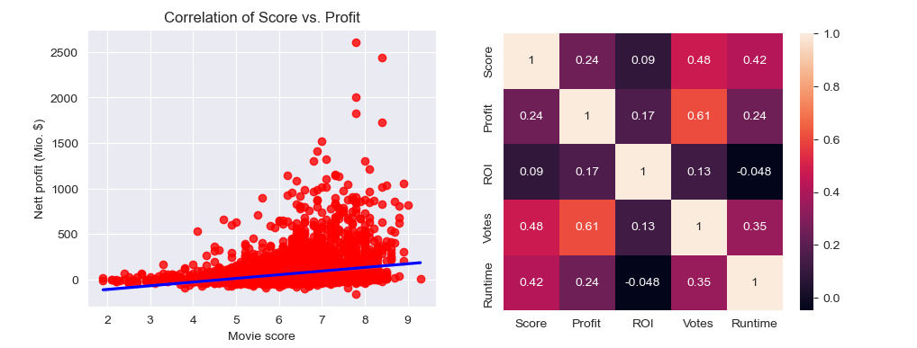
Since there are outliers in Profit axis, removing 5% outliers was expected to lead to higher correlation. However, the assumption was wrong, correlation even decreased!
# Will removing 5% outliers increase correlation?
q=df['Profit'].quantile(0.95)
df2=df[df['Profit'] < q]
fig = plt.figure(figsize = (5, 4))
sns.set_style("darkgrid")
#plot scatter graph
sns.regplot(x='Score',y=df2['Profit']/1000000, data=df2, scatter_kws={"color": "red"}, line_kws={"color": "blue"})
plt.xlabel('Movie score')
plt.ylabel('Nett profit (Mio. $)')
plt.title('Correlation of Score vs. Profit (removed outliers)')
# plot heatmap
sns.heatmap(df2[['Score','Profit','ROI','Votes','Runtime']].corr(), annot=True)
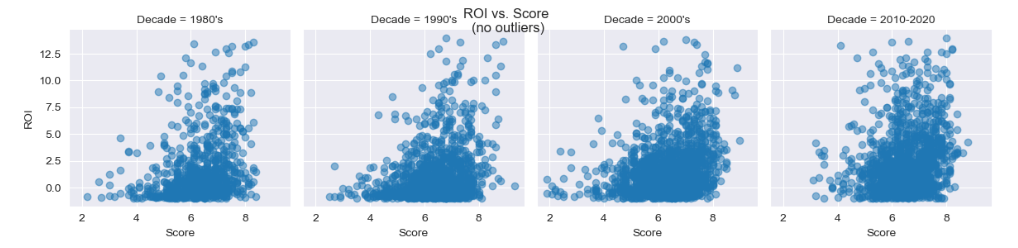
5-Multivariate analysis - over each decade find correlation of score vs. ROI
Find correlation between average movie score and return of investment (ROI) for each decade. ROI is the ratio between the nett profit and budget.
Scatter graphics show very small correlation between ROI and Score, for each of 4 decades.
g=sns.FacetGrid(data=df, col='Decade', col_wrap=4)
g.map(plt.scatter, 'Score', 'ROI', alpha=0.5)
g.fig.suptitle('ROI vs. Score')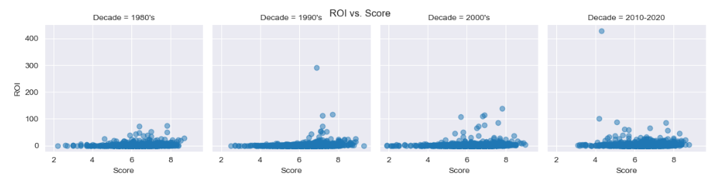
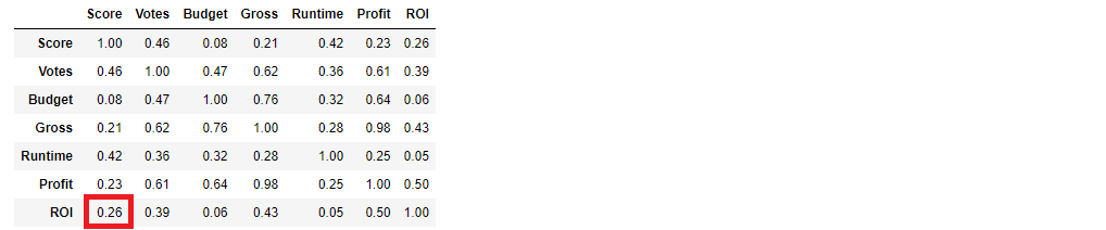
Correlation matrix shows correlation factor
df.corr(numeric_only =True) 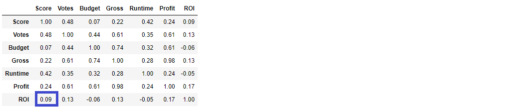
Removing only 3% of outliers in ROI axis signifficantly increased correlation!
# Will removing of 3% outliers change anything?
q=df['ROI'].quantile(0.97)
df2=df[df['ROI'] < q]
g=sns.FacetGrid(data=df2, col='Decade', col_wrap=4)
g.map(plt.scatter, 'Score', 'ROI', alpha=0.5)
g.fig.suptitle('ROI vs. Score \n(no outliers)')
Increased correlation factor can be obtained from correlation matrix as well
df2.corr(numeric_only =True) #removing 3% outliers increased correlation factor signifficantly!