Barry on Data Analysis

Python Web Scraping of German companies in Fortune Global 500

RESUME - Project overview

Jump to: SOLUTION -Project implementation

The data source is a Page on Wikipedia where there is a table with top 30 largest German companies, ranked in the Fortune Global 500 list as well. The Fortune Global 500, also known as Global 500, is an annual ranking of the top 500 corporations worldwide as measured by revenue. The list is compiled and published annually by Fortune magazine. The data will be loaded using Web Scraping method and after loading data will be analyzed to obtain useful insights.

Problem Statement

As Data Analyst searching for a job in Germany, I am interested in some details of top German companies. There are information available on Wikipedia Page, but I need some useful insights such as the most profitable industries, the most successful companies by profit per employee or the cities with more company headquarters. I would like to have these insight vizualized, but on Wikipedia there is only a table and some text, so I need a technique to obtain the Wiki table into data model that is able to be processed.

Skills & Concepts demonstrated

There are following Python & other features used in this project

Using libraries pandas, matplotlib and seaborn

Using bs4 library - BeautifulSoup constructor, find() and find_all() methods, element.Tag attributes

Using class_ argument of BeautifulSoup.find_all() method

Using requests library - method get() and attribute Response.text

Web page inspection for HTML tags <table>, <tr>, <th>, <td>

Using libraries pandas, matplotlib and seaborn

Plot visuals using Series.plot.bar(), seaborn.barplot(), matplotlib.pie(), seaborn.heatmap(), seaborn.regplot()

DataFrame construction from the column list and appending rows using loc[]

Convert string Series with negative numbers to numerical type

Function isdigit() for numerical character check

List comprehension

String functions strip(), replace()

Exporting DataFrame to CSV file using DataFrame.to_csv() method

Extracting largest values from DataFrame using nlargest() method

Rename DataFrame index using rename_axis() method

Data aggregation using groupby() and sum() methods

There are following insights I would like to get about the top 30 German companies:

Questions

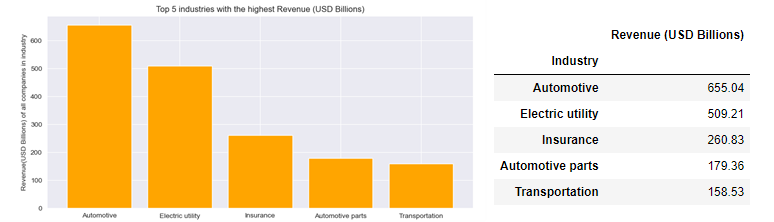
1-Which are the top 5 industries with the highest Revenue?

2-Find top 10 companies by profit per employee and visualize results along with company industries

3-Which cities are headquarters for 2 or more companies?

4-Categorize companies by Employee count (thresholds of 50,000, 100,000, 200,000 and 400,000) and find the 10 largest

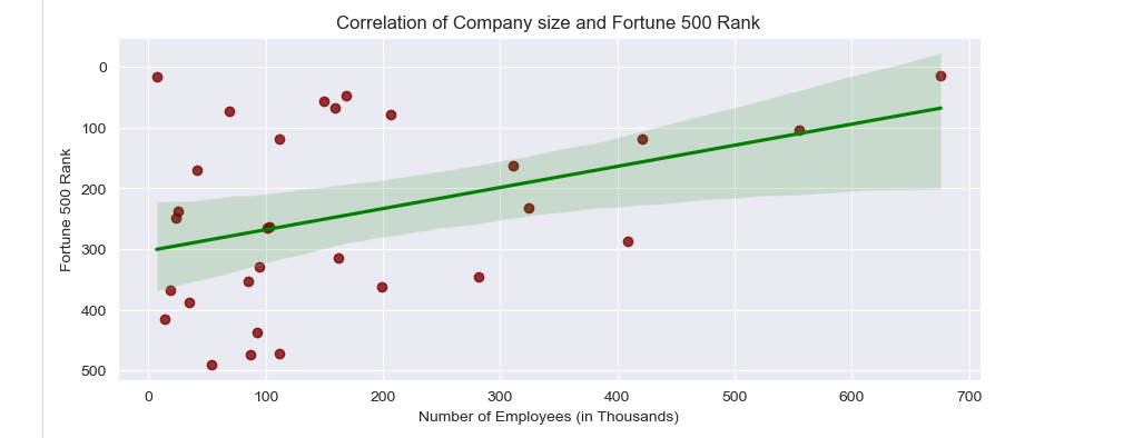
5-Find correlation between company size and Fortune 500 Rank

Insights

1. Among Top 30 largest German companies listed in the Global Fortune 500, the Industry with the highest cumulative Revenue in Billions of USD is Automotive industry (655), folowed by Electric utility (509), Insurance (261), Automotive parts (179) and Transportation (159).

2. The highest profit per employee in Thousands USD has Electric utilty company RWE (156). The 2nd best is BMW(126), followed by Mercedes-benz Group (90) and Munich Re (87). On the 5th place is Electric utiity company EnBW (72), followed by Deutsche Bank (67) and Talanx (52). On the 8th place is Allianz (45), followed bay Bayer (43) and Deutsche Telekom (41)

3. The city with most listed company headquarters is Munich (4), followed by Essen (3), Hanover (2), Hamburg (2), Stuttgart (2), Bonn (2) and Duesseldorf (2).

4. The most companies (9) have 100,000-200,000 employees, followed by companies (7) with less than 50,000 employees. On the 3rd place are the companies (6) with 50,000-100,000 employees, followed by companies (4) that have 200,000-400,000 employees and companies (4) with more than 400,000 employees.

The largest size company by employees (675,805) is Volkswagen, followed by Deutsche Post (554,975), Robert Bosch GmbH (421,338), Edeka Zentrale (408,900) and Deutsche Bahn (324,136). On the 6th place is Siemens (311,000), followed by Fresenius (282,024), Deutsche Telekom (206,759), Continental AG (199,038) and Mercedez-Benz Group (168,797)

5. The reasonable assumption was there is a high positive correlation between company size and Fortune Global 500 Rank. However, it shows up that correlation is positive, but not so high as expected:

SOLUTION - Project implementation

Back to: RESUME -Project overview

0.1-Inspecting Data source

0.2-Importing libraries and loading HTML page

0.3-Extracting table and loading from HTML to DataFrame

0.4-Data Transformation

0.5-Exporting Data to CSV file

1-Top 5 industries with the highest Revenue

2-Top 10 companies by profit per employee and their industries

3-Which cities are headquarter for 2 or more companies

4-Categorize companies by Employee count and find the 10 largest

5-Find correlation between company size and Fortune 500 Rank

Before processing business questions, there is Web Page to be loaded into data model using Web Scraping in Python.
On the GitHub Repository there is Jupyter Notebook script available.

0.1-Inspecting Data source

Dataset is table on Wikipedia Page that contains column of Fortune Global 500 Rank.

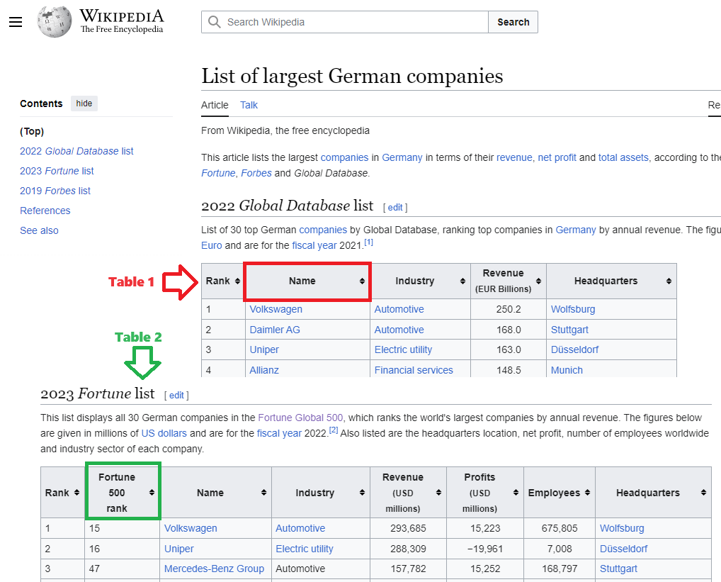
Using Inspect option on the Right-click menu browser will open HTML view of the page on the right side. Especially useful for inspecting web page is selecting the option shown below with number 2, as it will highlight the right position within HTML source (on the right side) on selection a particular element (table or whatever else) on the web page (on the left side).

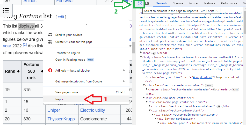
The web page inspection gets the following insights

The required table has 30 rows + header and 8 columns

There is one table before the required one, the table we need is in the 2nd position

There is column Nr. 2 that is different: "Fortune 500 Rank" is in the table we need

Table class is 'wikitable sortable'

0.2-Importing libraries and loading HTML page

Beautiful Soup is a Python library for scraping data from websites. Requests is an HTTP client library for the Python programming language. We need to import both of them for this project, as well as pandas library for the phase when it will be started to use DataFrame. Loading of the HTML page is done using requests.get() method, that gets URL as parameter and returns Response object. In this case, the return code is 200, which ist standard HTTP success status response code that indicates that the request has succeeded.

from bs4 import BeautifulSoup
import requests
import pandas as pd
url='https://en.wikipedia.org/wiki/List_of_largest_German_companies'
page=requests.get(url)
type(page), page

Using text attribute there is a content of the returned object, which is not pretty formatted HTML, and it will look better by using Beatiful Soup.

page.text

The constructor of BeautifulSoup object gets Response object and parser specification as arguments. Quick check shows there is BeautifulSoup object created.

soup=BeautifulSoup(page.text, 'html.parser')
type(soup)

Printing content of the BeautifulSoup object shows slightly better HTML formatting, although far from useful or human-readable.

soup

Using text attribute of the element.Tag class there can be extracted title of loaded HTML page:

type(soup.title), soup.title.text

0.3-Extracting required Data table

For searching within HTML there 2 methods: find() returns the first object with specified tag, and find_all() returns all objects that have specified tag as a list (accessible by list indexing).

Table in HTML is defined with <table> tag.

Table row within HTML table is defined with <tr> tag.

Table header within HTML row is defined with <th> tag.

Table data row within HTML row is defined with <td> tag.

The results of the find() method show the first table on Wiki Page, which is not the one that we need:

soup.find('table') # returns the first table only, but we need the second table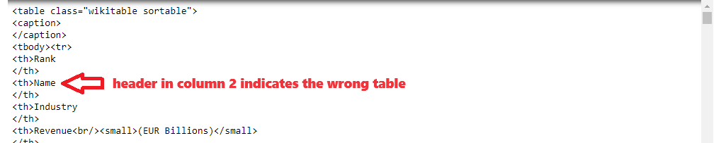

The table we need will be accessed as the second element of the returned list

table = soup.find_all('table')[1] # returns 2nd list element - that's the table we need!
table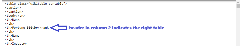

In case there are more table classes in HTML page, it can be explicitly specified particular table class using _class parameter:

table == soup.find_all('table', class_='wikitable sortable')[1] # list of tables using table class - compare

Once table is found, loading to DataFrame will be done in 2 steps: loading table headers that will define DataFrame columns, and after that loading table data rows and appending them to the table

Loading table headers

To load table headers it will be used find_all() method that returns a list:

#get table headers
table_headers = table.find_all('th')
print(table_headers)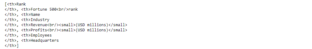

Using list comprehension and text attribute, the HTML tags will be removed:

table_titles = [title.text for title in table_headers] # cleaning from HTML tags 
print(table_titles)

Using string method strip() newline characters will be removed:

table_titles = [title.text.strip() for title in table_headers] # cleaning from newline escape sequences 
print(table_titles)

The final clean list will be loaded to DataFrame as column names:

df= pd.DataFrame(columns=table_titles) #loading column headers
df

Loading table data rows

Table data rows will be built out of each piece of data found within each particular table row, using find_all() method:

table_rows=table.find_all('tr')
for row in table_rows:
    data_rows = row.find_all('td')
    table_data_row=[title.text.strip() for title in data_rows]
    print(table_data_row)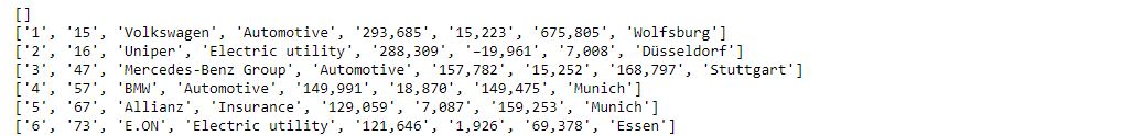

Since there is a table header found, looping through the list and loading data to DataFrame will be strated from 2nd list element (skipping headers):

# insert the data rows into DataFrame
for row in table_rows[1:]: # skip the first row that is header
    data_rows = row.find_all('td')
    table_data_row=[title.text.strip() for title in data_rows]
    length=len(df) # new row's index in the DataFrame will be equal to DataFrame row count before adding new 
    df.loc[length]=table_data_row
df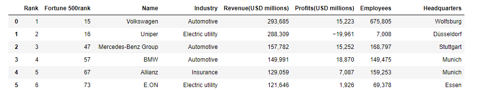

Now there is a table from Wikipedia Page loaded into the DataFrame object!

0.4-Data Transformation

Although there is a very small-sized Dataset, it's good practice to check NULL values and duplicates. Since there aren't any, there's no need for Data Cleaning as well.

df.isnull().sum().any(), df.duplicated().any()

After successful loading data into DataFrame, all the columns are the 'object' type by default. There are 2 types of columns in this table: numerical (integer) and string, and all columns will be converted accordingly.

df.info()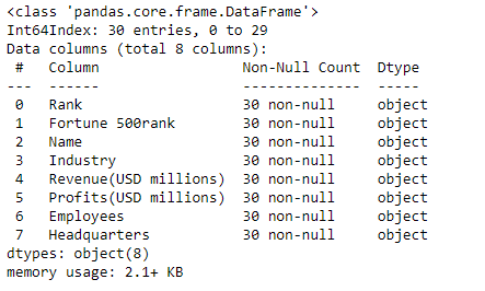

Numeric column type conversion

The first try of numeric column conversion failed!

# Conversion to integer - Try No. 1
lsNumCols = ['Rank', 'Fortune 500rank', 'Revenue(USD millions)', 'Profits(USD millions)', 'Employees']
df[column] = [df[column].astype('int32') for column in lsNumCols]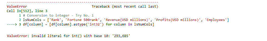

The cause of error raised is comma within string numeric data.
However, after removing commas the conversion failed again! What's wrong?

# Conversion to integer - Try No. 2 - Remove commas from string numbers
for column in lsNumCols:
    df[column] = df[column].str.replace(',','')
    df[column] = df[column].astype('int32')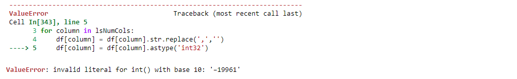

The reason of this error raised lies in negative numbers. If negative numbers are stored with Unicode minus (code point '\u2212' or decimal 8722) or hyphen (code point '\u2010' or decimal 8208) conversion is not possible. The solution is to replace the current minus sign with the standard minus sign, and conversion is done!

# Conversion to integer - Try No. 3 - Remove commas and Ensure standard minus sign instead of unicode hyphen/minus sign
def MakeProperStrNumSeries(sColumnName):    
    df[sColumnName] = df[sColumnName].astype(str) # convert column to string    
    df[sColumnName] = df[sColumnName].str.replace(',','') # remove comma to be able to convert to number       
    lsItems=df[sColumnName].tolist() #convert Series to list
    lsNum = [] #list of numerical values to append after conversion

    for item in lsItems:
        item = item.strip() #remove leading and trailing blanks if there are any
        if(item[0].isdigit() == False): # if not digit, it has to be minus             
            item=item.replace(item[0],'-') # replace unicode minus/hyphen sign with standard minus sign            
        n=int(item) 
        lsNum.append(item)        
        
    df[sColumnName]=pd.Series(lsNum) 

# Convert string column to numeric column properly
def StrColumnToNumber(sColumnName):
    df['colHelper'] = df[sColumnName] # helper column 
        
    # For negative numbers, ensure there is standard minus sign
    MakeProperStrNumSeries('colHelper')     
    
    df['colHelper'] = df['colHelper'].astype('int32') # convert to integer
    df[sColumnName] = df['colHelper']
    df.drop(columns='colHelper', inplace=True) #remove helper column

# call function in the columm list comprehension
[StrColumnToNumber(column) for column in lsNumCols]
df.info()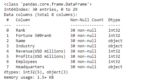

String column type conversion

String columns conversion is done successfully.

#Convert string columns
lsStrCols = ['Name', 'Industry', 'Headquarters']
for column in lsStrCols:
    df[column] = df[column].astype('string')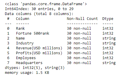

0.5-Exporting Data to CSV file

DataFrame will be exported to CSV file using to_csv() method. Index parameter is set to False since there's no need for additional column.

df.to_csv('C:/Users/User/OneDrive/Documents/BLOG/Portfolio/webScrapeExport.csv', encoding='utf-8', index = False)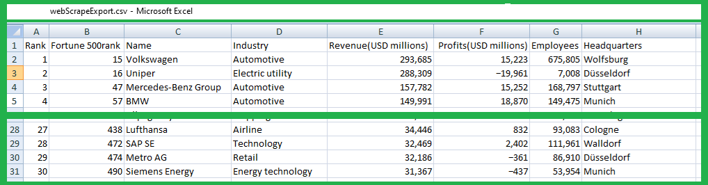

1-Top 5 industries with the highest Revenue

The required Data subset is extracted from the DataFrame using groupby() method and sum() aggregate function on Series object. Visualization is done using Series.plot.bar() method.

import seaborn as sns
import matplotlib.pyplot as plt
seriesSum =df.groupby('Industry')['Revenue(USD millions)']
seriesSum = seriesSum.sum()/1000 # show in USD Billions
seriesSum = seriesSum.sort_values(ascending=False).head(5) # sort values Descending and take top 5
dfTop5 = pd.DataFrame(seriesSum)
dfTop5.rename(columns={'Revenue(USD millions)': 'Revenue (USD Billions)'}, inplace=True)
# plot bar chart
plt.figure(figsize=(11,5))
sns.set_style('darkgrid')
seriesSum.plot.bar(color ='orange', width=0.8)
plt.xlabel("")
plt.ylabel("Revenue(USD Billions) of all companies in industry")
plt.title("Top 5 industries with the highest Revenue (USD Billions)")
plt.xticks(rotation=0)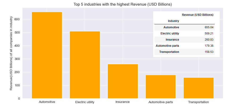

2-Top 10 companies by profit per employee and their industries

Data subset is extracted using nlargest() method after sorting and visualized using seaborn.barplot() method.

df['ProfitPerEmployee (USD Thousands)'] = df['Profits(USD millions)'] / df['Employees'] * 1000 # Thousand  USD
pd.set_option('display.float_format', lambda x: '{:,.2f}'.format(x)) # format float as 1,000.00
colNames=['Name','ProfitPerEmployee (USD Thousands)','Industry', 'Profits(USD millions)','Fortune 500rank', \
          'Employees', 'Headquarters']
top10_rated=df.nlargest(10,'ProfitPerEmployee (USD Thousands)')[colNames].set_index('Name')
top10_rated['Employees'] = top10_rated['Employees'].apply(lambda x: '{:,}'.format(x)) # format integer as 1,000
top10_rated['Profits(USD millions)'] = \
            top10_rated['Profits(USD millions)'].apply(lambda x: '{:,}'.format(x)) # format integer as 1,000
top10_rated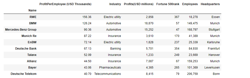

plt.figure(figsize=(8,4))
sns.barplot(x='ProfitPerEmployee', y=top10_rated.index, data=top10_rated,hue='Industry', dodge=False)
plt.xlabel("Profit Per Employee (Thousand USD)")
plt.ylabel("Company")
plt.title("Top 10 companies with the highest Profit per employee and their industry")
plt.legend(bbox_to_anchor=(1.02,1),loc=2)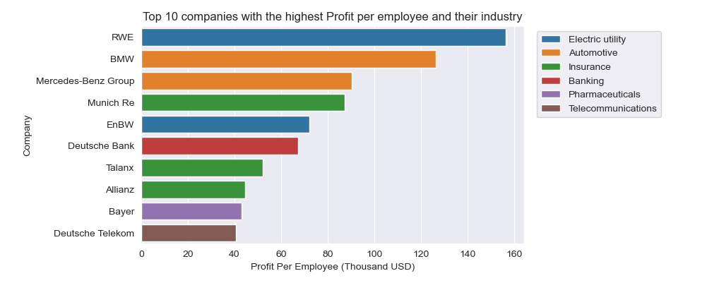

3-Which cities are headquarter for 2 or more companies

Dataset required is extracted using value_counts() method, directly passed as boolean index to the DataFrame object and selected particular Series. Visualization is done using Series.plot.bar() method.

plt.figure(figsize=(12,3))
plt.title('Headquarters with 2 or more companies')
      
df2 = pd.DataFrame(df['Headquarters'].value_counts() )
series2= df2[df2['Headquarters'] > 1]['Headquarters']
series2.plot.bar(color ='purple', width=0.85) 

plt.xticks(rotation=0)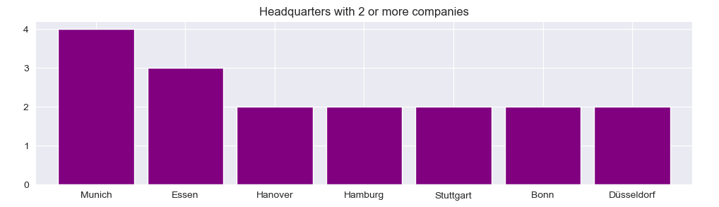

4-Categorize companies by Employee count

Data categorization is done using cut() method. For Company categorization by company size it is added new column and visualized with pie chart. For the pie chart it has to be prepared list containing item count for each category.

lsLimits= [0,50000,100000,200000,400000,800000]
lsBinLabels = ['Up to 50,000 Employees', 'From 50,000 to 100,000 Employees', 'From 100,000 to 200,000 Employees',\
                'From 200,000 to 400,000 Employees', 'More than 400,000 Employees']
df['Size']=pd.cut(df['Employees'], lsLimits, labels=lsBinLabels, include_lowest=True)

nCatCount=[]
for label in lsBinLabels:
    nCatCount.append(len(df[df['Size'] == label]))
    
lsLabels = []
lenList = len(lsBinLabels) 
for i in range(lenList):       
    lsLabels.append(lsBinLabels[i] + ' (' + str(nCatCount[i]) + ')')

fig, ax = plt.subplots()
ax.pie(nCatCount, labels=lsLabels, autopct='%1.1f%%')
plt.title('Company categories by size (Employee count)')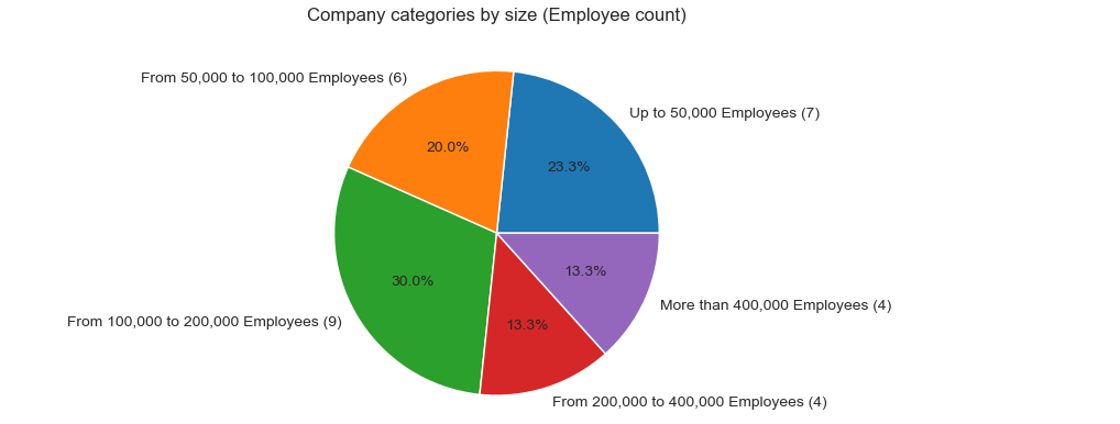

Top 10 companies by size are extracted using nlargest() method, and index is renamed using rename_axis() method. Data are visualized by vertical bar chart by passing parameter orient = 'v' to the seaborn.barplot() method:

top10_emp=df.nlargest(10,'Employees')[['Name','Employees', 'Industry']].set_index('Name')
top10_emp_show=top10_emp.copy()
top10_emp_show['Employees'] = top10_emp_show['Employees'].apply(lambda x: '{:,}'.format(x)) # format integer as 1,000
top10_emp_show.rename_axis('Company', inplace=True) # rename index
top10_emp_show[['Employees']]
# plot bar
plt.figure(figsize=(9,3))
sns.barplot(y=top10_emp['Employees']/1000, x=top10_emp.index, data=top10_emp, orient='v', hue='Industry', \
            width=0.9, dodge=False)
plt.ylabel("Employees (in Thousands)")
plt.xlabel("")
plt.title("Top 10 largest German companies")
plt.legend(bbox_to_anchor=(0.7,1),loc=2)
plt.xticks(rotation=45)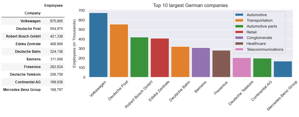

5-Find correlation between company size and Fortune 500 Rank

The assumption is, since Fortune Global 500 rank list is based on company revenue, that there will be a very high correlation between company size and Fortune 500 Rank as well. As lower Fortune 500 Rank value in the data model means the higher rank, it makes sense to extend data model with Reversed Rank column, to gett better visual insight of the correlation. The correlation (relationship) between each column in the DataFrame are found using corr() method, with the default Pearson methodology.

df['F500rank Reversed'] = 500 - df['Fortune 500rank'] # extend DataFrame with reversed Rank column
dfcorr=df.corr(numeric_only =True)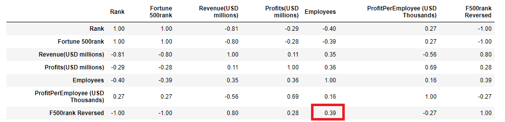

The assumption was not completely right, the correlation (factor=0.39) is positive but still belongs to the Low positive correlation category. There is and interpretation of correlation factors:

0.9 to 1.0 (-0.9 to -1.0) -Very high positive (negative) correlation

0.7 to 0.9 (-0.7 to -0.9) -High positive (negative) correlation

0.5 to 0.7 (-0.5 to -0.7) -Moderate positive (negative) correlation

0.3 to 0.5 (-0.3 to -0.5) -Low positive (negative) correlation

0.0 to 0.3 (0.0 to -0.3) -Negligible correlation

Using seaborn heatmap correlation factors can be visualized:

plt.figure(figsize=(10,4))
sns.heatmap(dfcorr, annot=True, cmap="Blues")
plt.xticks(rotation=45)
plt.title('Correlation Heatmap (Pearson method)')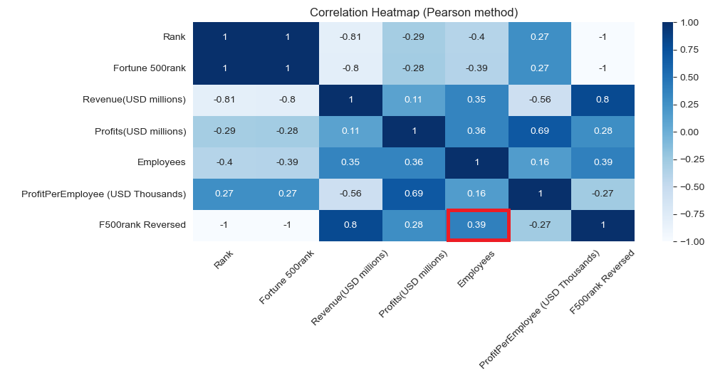

Finally, the seaborn scatter plot visualizes the bivariate analysis:

fig = plt.figure(figsize = (10, 4))
#plot scatter graph
sns.set_style("darkgrid")
ax=sns.regplot(x=df['Employees']/1000, y=df['Fortune 500rank'], data=df, scatter_kws={"color": "maroon"}, \
                line_kws={"color": "green"})
ax.invert_yaxis() # Rank values in Reversed order
plt.xlabel('Number of Employees (in Thousands)')
plt.ylabel('Fortune 500 Rank')
plt.title('Correlation of Company size and Fortune 500 Rank')

About the author

Barry The Analyst has been working from May 2022 untill July 2023 with one big company in Ireland, and since July 2023 has worked with one big company in Germany. This blog was started as a private note collection in order to (re)develop, refresh and strengthen essential skills of Data Analysis field. The content was generated on the way of learning path, with a degree in Electrical Engineering and experience in C++/SQL. Private notes turned into public blog to share the knowledge and provide support to anyone who would find this interesting...

Who is this for?

This is not yet another basic course that would explain elementary concepts. There are many basic features of tools and technologies that are skipped in blog articles and portfolio projects here presented. If you are not an absolute beginner in SQL/databases, Excel, Python and Power BI this might be useful material if you would like to advance a career as Data Analyst and/or Python Developer ...

Barry on Data Analysis-brief insights to relevant facts, definitions and best practices-