


RESUME - Project overview
Jump to: SOLUTION -Project implementation
Skills & Concepts demonstrated
The data source is Excel workbook containing data about coffee sales during the period 2019-2022. There is a list of orders, customers and products in each particular worksheet.
Problem Statement
The goal of this project is to analyze the Coffee Sales dataset and derive valuable insights about the sales of different types of coffee to different destinations and find what types of coffee are more popular than others. The main worksheet in the Excel workbook Dataset contains 1,000 rows with coffe order data.
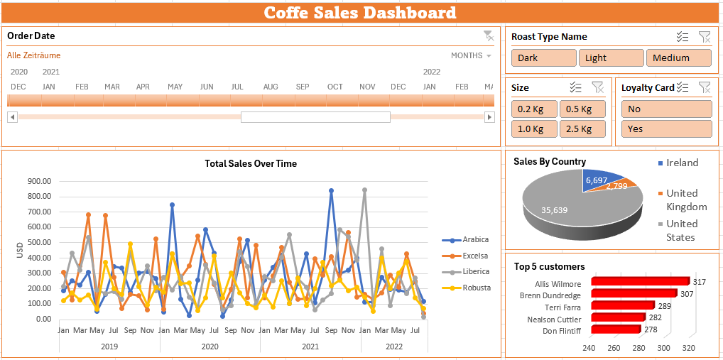
There is Dashboard to be built in order to be able to get insights i.e. answers to particular business questions, as well to enable a flexibility and opportunity answering to possible future questions using interactive Dashboard's user interface.
Skills & Concepts demonstrated
There are following Excel features used in this project
There are following insights needed to be obtained:
Questions
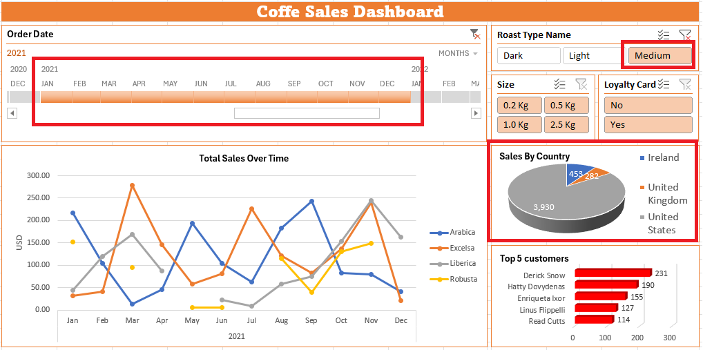
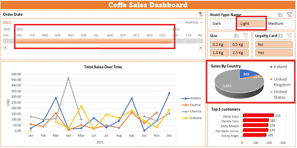
1-For each particular Roast type, what is total Sales by country in 2021 year?
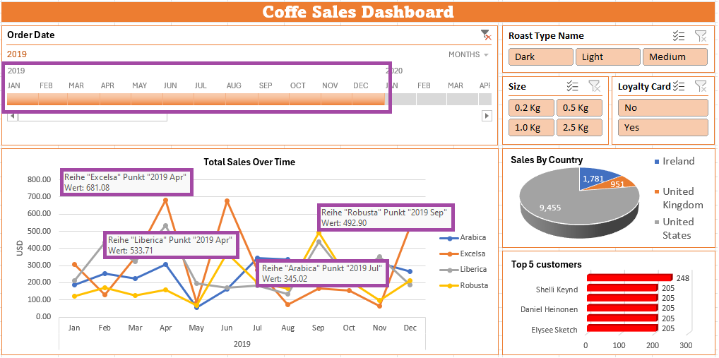
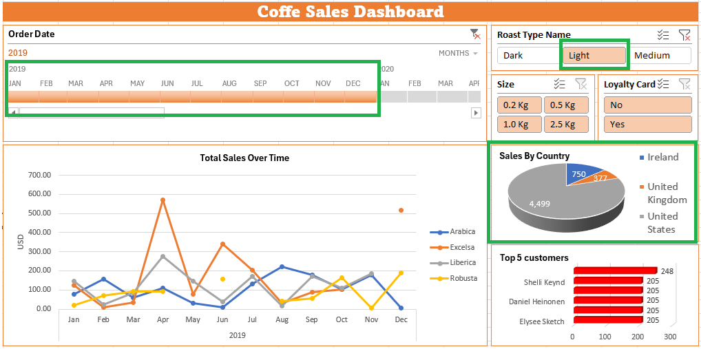
2-What was the top month by coffee sales for each coffe type in the year 2019?
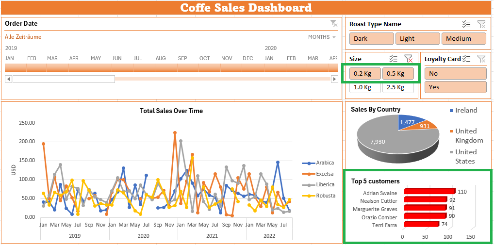
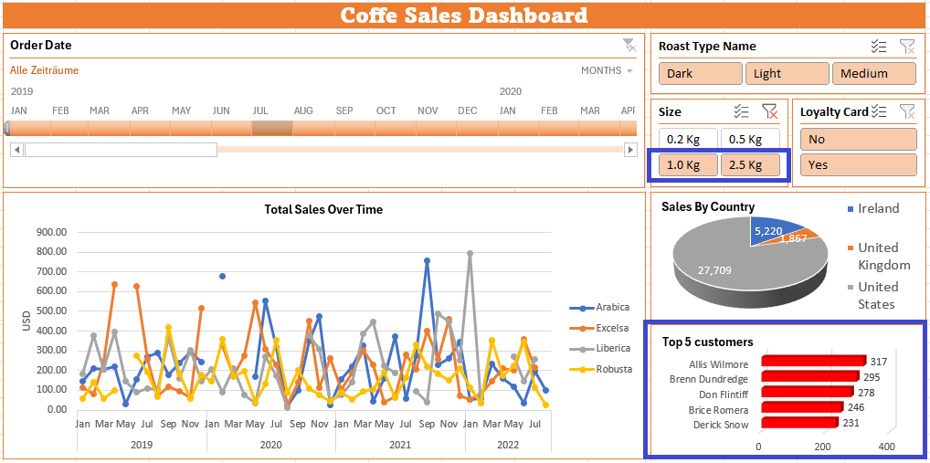
3-For pack Size group below 1 kg and 1 kg or above, which are the top 5 customers overall?
4-Which was the most popular Roast type in Ireland for each particular year?
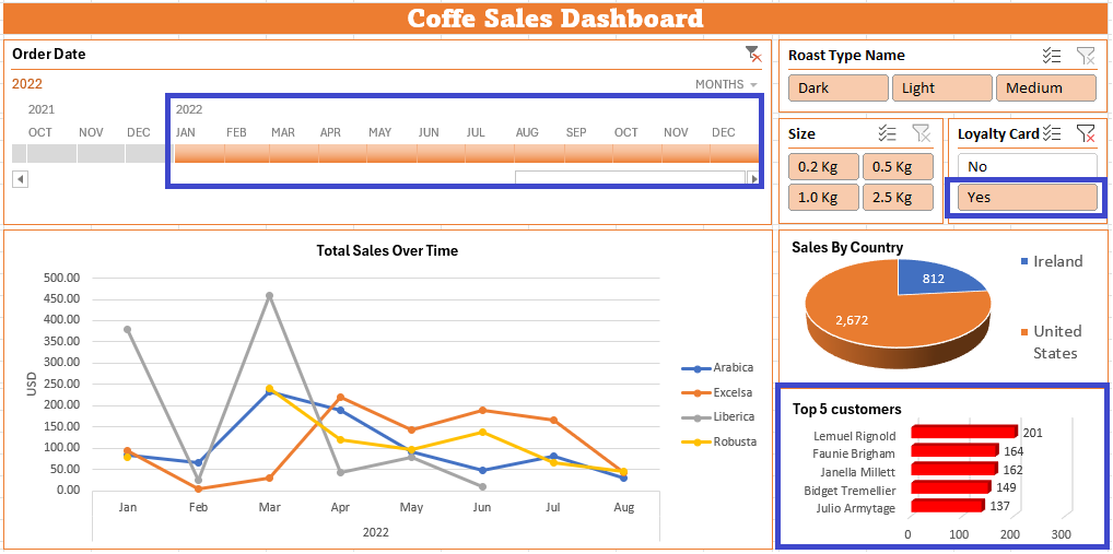
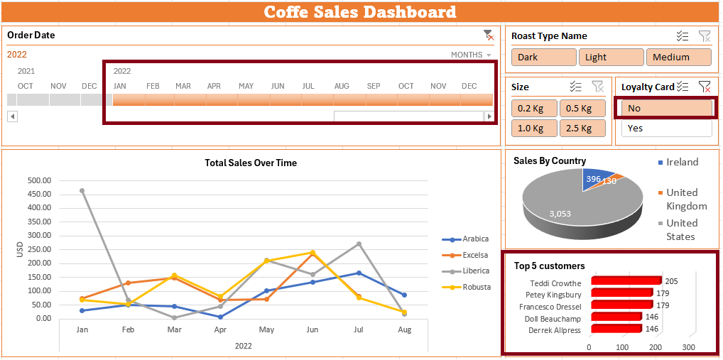
5-Which are top 5 customers of the 2022 year with Loyalty card and without it?
Insights
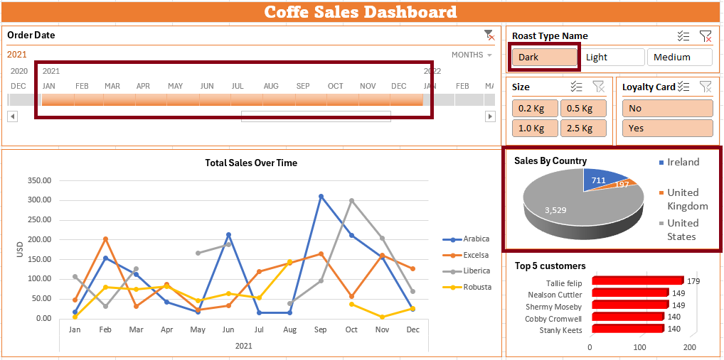
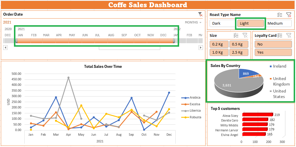
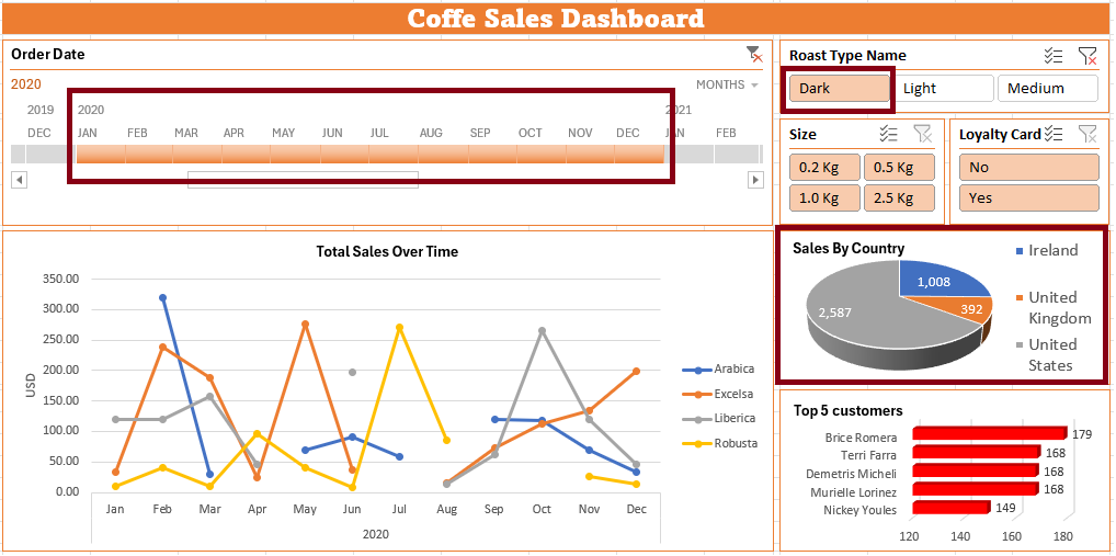
1. In the year of 2021, For the Dark Roast type there is the highest Sales in USA ($ 3,529) followed by Ireland ($ 711) and UK ($ 197). The Light Roast type is sold the most in USA ($ 3,631) followed by Ireland ($ 869) and UK ($ 164). The Medium Roast type was the most popular again in USA ($ 3,930), followed by Ireland ($ 453) and UK ($ 282)


2. In the year 2019 the top month per coffe type was the following:
3. The Top 5 customers overall for small pack sizes (0.2kg and 0.5kg) as well as for big pack sizes (1kg and 2.5kg):

Small pack sizes - The top customer is Adrian Swaine ($ 110), followed by Nealson Cuttler ($ 92) and Marguerite Graves ($ 91). The 4th position belongs to Oracio Comber ($ 90), followed by Terri Farra ($ 74)

Big pack sizes - The top customer in this group is Allis Wilmore ($ 317), followed by Brenn Dundredge ($ 295) and Don Flitiff ($ 278). The 4th position belongs to Brice Romera ($ 246), followed by Derick Snow ($ 231)
4. The most popular roast type in Ireland year-wise was the following:
5. In the year 2022 there are following top 5 customers breakdown by Loyalty card:

Customers with Loyalty Card - The top customer is Lemuel Rognold ($ 201), followed by Faunie Brigham ($ 164) and Janella Millet ($ 162). The 4th position belongs to Bidget Tremellier ($ 149), followed by Julio Armytage ($ 137)

Customers with No Loyalty Card - The top customer in this group is Teddi Crowthe ($ 205), followed by Petey Kingsbury and Francesco Dressel who share the 2nd position with the same amount spent ($ 179). Also the position 4 is shared between Doll Beauchamp and Derrek Allpress ($ 146)
SOLUTION - Project implementation
Back to: RESUME -Project overview
0.1-Populating columns using XLOOKUP and INDEX MATCH
0.3-Visualisation using Line chart, Bar chart and Pie chart
0.4-Creating Timeline and Slicer objects
0.5-Building interactive Dashboard
1-Total sales by country in 2021 breakdown by Roast type
2-Top month in year 2019 for each coffee type
3-Breakdown by pack size and find top 5 customers overall
4-For Ireland find the most popular Roast type year-wise
5-Top 5 customers in 2022 with/without a Loyalty card
The raw data model has to be extended and objects have to be created in order to build an interactive Dashboard and to be able to get required insights.
There are on the GitHub Repository available:
0.1-Populating columns using XLOOKUP and INDEX MATCH
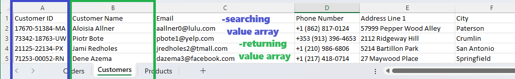
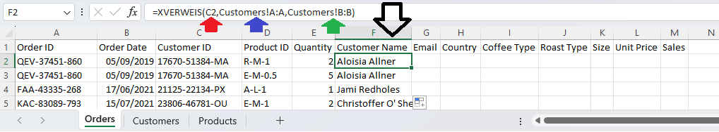
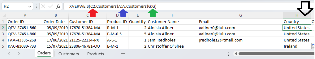
The columns Customer Name, Email and Country in the Orders worksheet have to be populated by searching data from the worksheet Customers, and it will be accomplished using XLOOKUP (XVERWEIS) function. The columns Coffee Type, Roast Type, Size and Unit Price have to be populated with values fro the Products worksheet that will be accomplished using INDEX MATCH (INDEX VERGLEICH) function combination. Finally, column Sales will be populated using simple calculation as product of Unit Price and Quantity columns.
XLOOKUP (XVERVEIS) function
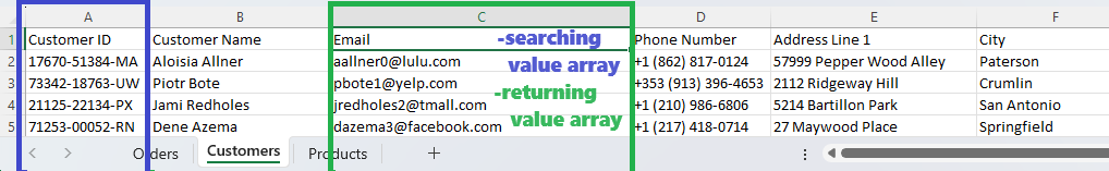
For columns Customer Name, Email and Country the value searching for is the same as well the searching value array. The only difference is in the 3rd parameter i.e the returning value array, that depends on the column.
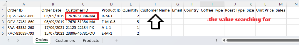
Using XLOOKUP function (XVERWEIS) data will be populated properly, passing as the 1st parameter the value searched, the 2nd parameter the array where is it looked for and the 3rd parameter the array from which the value will be returned.
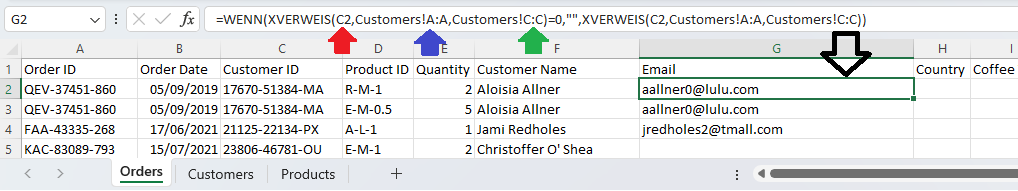
The column Email will be populating by wrapping the XLOKUP function in the nested IF function (WENN verkettet), in which it will be defined an empty string to be returned since some rows of e-mail addresses column are empty.
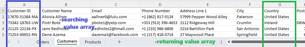
The column Country will be populated the same way as the column Customer:
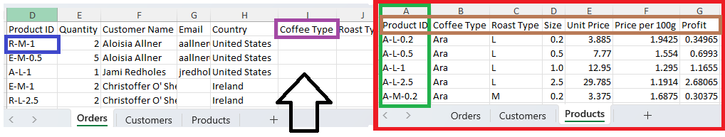
INDEX MATCH (INDEX VERGLEICH) function combination
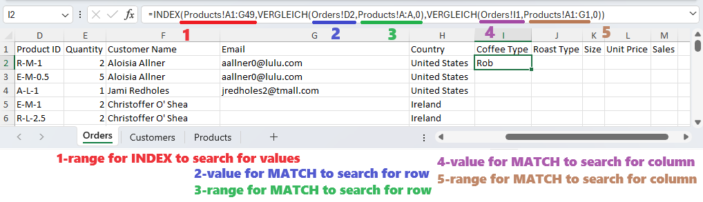
The next step is population columns Coffee Type, Roast Type, Size and Unit Price. It will be done using INDEX MATCH Excel tool (INDEX VERGLEICH). INDEX MATCH is very popular Excel tool and these 2 function are very efficient working together. INDEX function needs numeric positions of row and column of a passed range, and within INDEX there is nested MATCH function which finds those positions based on passed value.
The first column to be populated is CoffeeType.
The solution below gets correctly the value for the first cell.
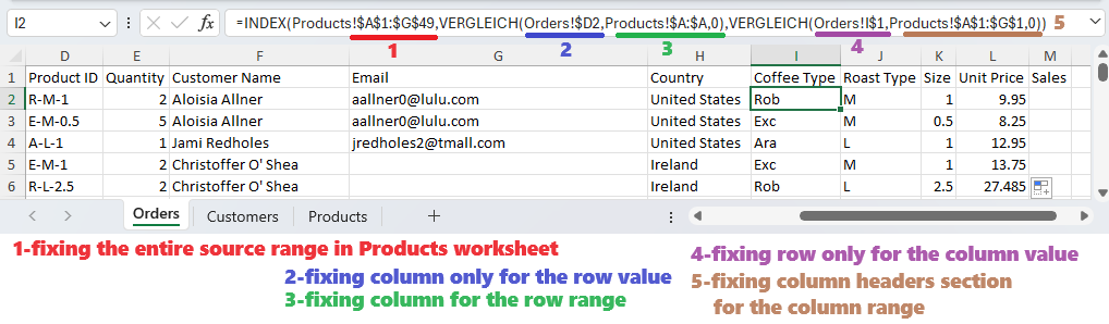
However, it would be not possible to populate entire column and to populate another 3 columns using the same formula. Excel is powerful enough to enable to populate cells dynamically with few modification i.e. fixing some parts of the formula. After fixing some formula section, all required columns will be populated:
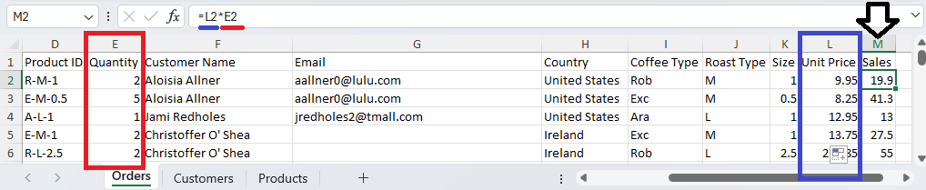
Populating table column using simple formula for product
The column Sales is populated using formula to multiply price and quantity:
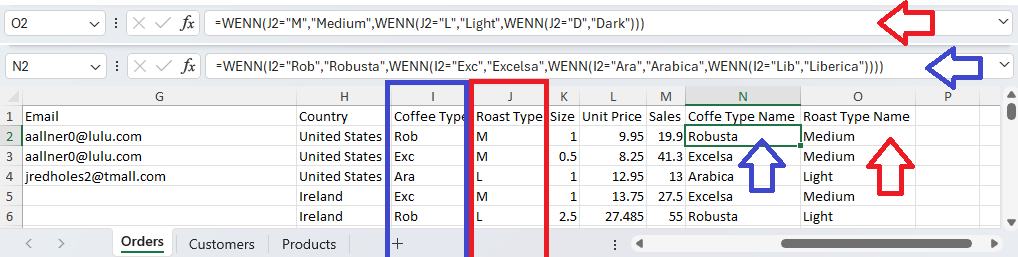
Adding new column using nested IF
Using nested IF (WENN verkettet), it will be added columns with full coffe type and roast type names.
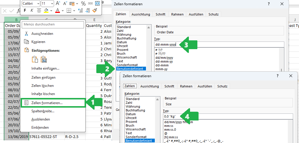
Formatting columns
The Date column will be formatted to see short month names. Selecting column and right-click to it will show pop-up menu with an option Zellen formatieren (1). In the dialogue box under Kategorie option it has to be selected Benutzerdefiniert (2) and entered custom date format (3). The Size column will be formatted to be shown units (kg). The dialogue box Format cells (Zellen formatieren) can be also opened by Ctrl+1. The "Kg" added to number has to be entered with quotation marks (4)
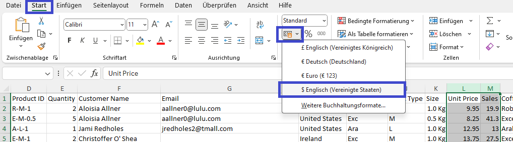
The columns Unit Price and Sales will be formatted in currency format. Affter selecting both column there is within Home(Start) menu the button that opens submenu for currency format selecting
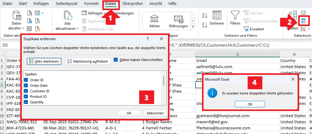
Removing duplicates will be done within Daten menu (1) by selecting Remove duplicates button (Duplikate entfernen) (2). The dialogue box will enable to select particular columns as criteria for duplicate detecting (3) and since there were no duplicates found the message box will show the results (4)
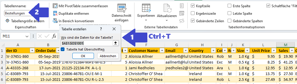
The range will be converted to table which is much more powerful feature since it dinamically recognizes adding or removing columns or formulas, which is especially useful in Pivot tables. While positioned in any range cell and pressing Ctrl+T table will be created out of entire range. It is good practice to give the table a meaningful name as well (2)
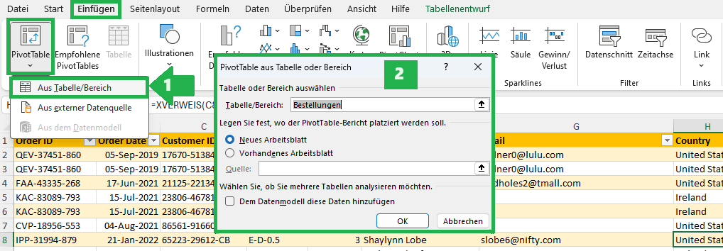
0.2-Creating Pivot table
Pivot table is created under Einfügen menu by selecting Pivot Table button. Since the data source is internal table, by selecting option Aus Tabelle/Bereich it will be offered the existing table Bestellungen. After confirmation a new empty Pivot table is created on the new worksheet.
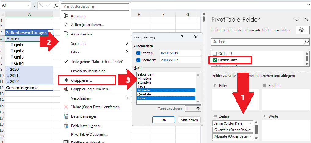
The first field to add to the pivot table is Date into the Rows (Zeilen) section (1). Date will be formatted to be shown only month and year, in a Tabular view. After right click on the date item in Pivot table there is menu offered (2) and it has to be selected option Gruppieren (3) to enable customized date formatting
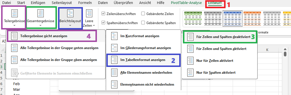
To customize Pivot Table layout there is Entwurf menu (1) that is available when Pivot Table selected. To show table in tabular form there is an option Im Tabellenformat anzeigen (2) within menu opened by selecting Berichtslayout button. To deactivate showing of totals and subtotals there is an option Für Zeilen und Spalten deaktiviert (3) within menu opened by selecting Gesamtergebnisse button as well as an option Teilergebnisse nicht anzeigen (4) within menu opened by selecting Teilergebnisse button
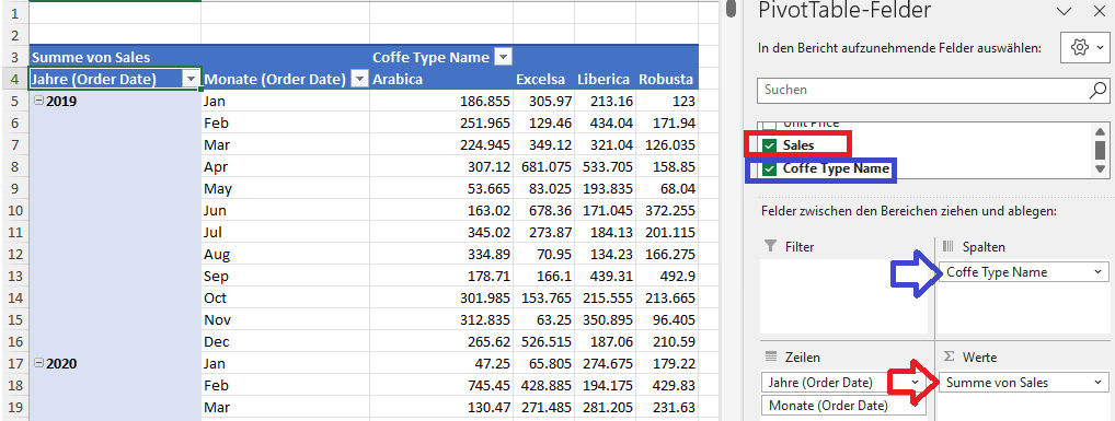
The next 2 fields to be added into Pivot Table is Coffe Type Name in the Columns (Spalten) section as well as Sales field into the Values (Werte) section
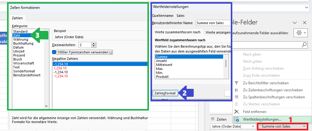
In order to format values properly by clicking the field in particular section it has to be selected Wertfeldeinstellungen option (1). In the dialogue box opened it has to be clicked the Zahlenformat button (2) and in Kategorie-Zahl (3) the proper formatting is to be defined:
0.3-Visualisation using Line chart, Bar chart and Pie chart
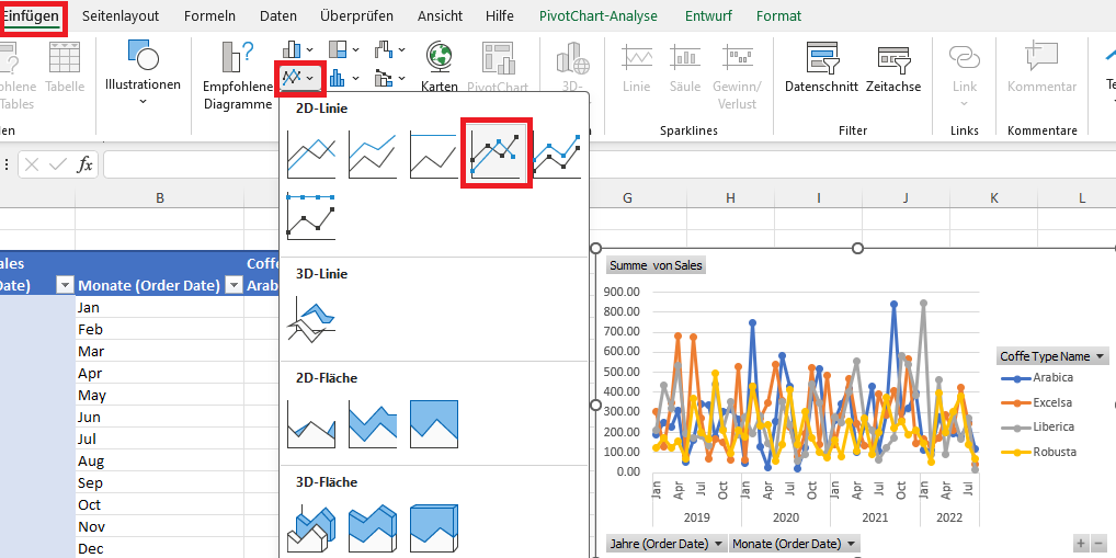
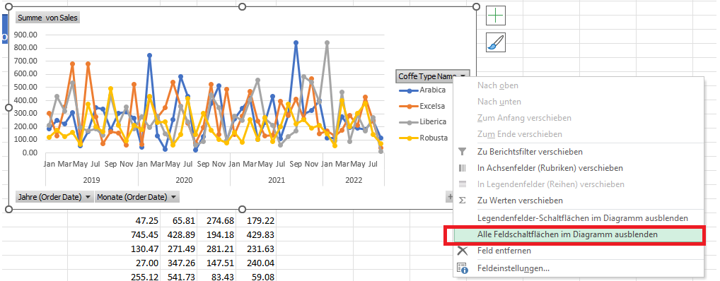
To insert line chart when selected any field in the Pivot Table under Einfügen menu it has to be selected Linie mit Datenpunkten option:
Removing field button is done by right-click on any field button in the chart and then selecting an option Alle Feldschaftflächen im Diagramm ausblenden:
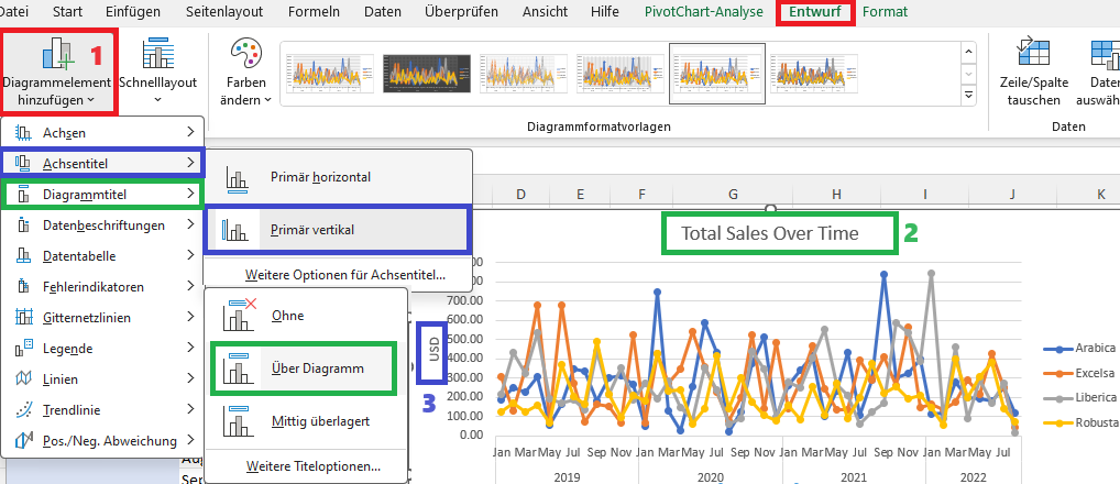
Adding axis titles and title to the chart is to be done in Entwurf menu by selecting button Diagrammelement hinzufügen (1). For diagram title there is option Diagrammtitel-Über Diagramm (2) and for the Y-axis title there is option Achsentitel-Primär vertikal (3)
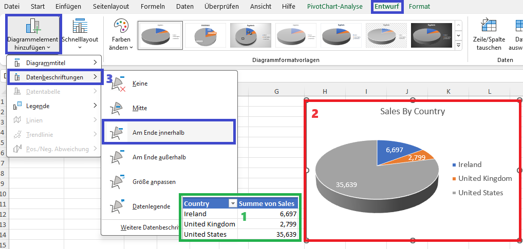
PieChart (2) will be created to vizualize Sales By Country. Pivot table as Data source (1) will be copied and in the field list there will be Country in Rows section and Sum of Sales in Values section. By default, Pie Chart does not have Data Labels, so it will be created using option Entwurf-Diagrammelement hinzufügen-Datenbeschriftungen (3)
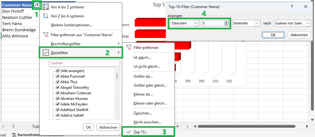
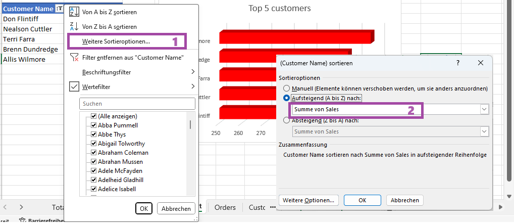
BarChart will be created to vizualize Top 5 customers. Pivot table as Data source will be copied and in the field list there will be Customer Name in Rows section and Sum of Sales in Values section. We don't need all the customers, just top 5 sorted. Selection of top 5 will be done using filter, by clicking button in the column header (1), then selecting Wertefilter option (2). After clicking Top 10...option (3) it has to be defined top 5 by entering 5 in Obersten option (4) By default, Bar Chart has legend but we don't need it so it will be removed.
Sorting items will be accomplished by selecting Weitere Sortieroptionen (1), then selecting radio button Aufsteigend (A bis Z) nach: (2) and select the column to sort by:
0.4-Creating Timeline and Slicer objects
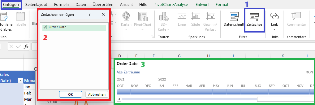
To insert Timeline object (3) it has to be selected in Einfügen menu the button Zeitachse (1), as well as to be selected Pivot Table in the dialogue box (2)
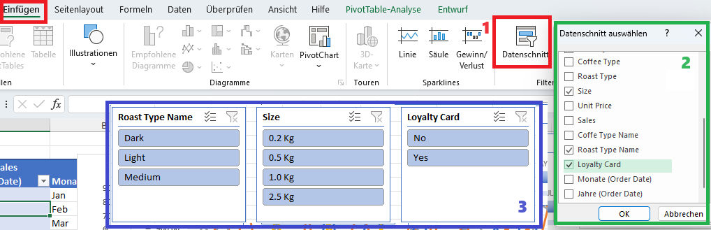
There are 3 Slicer objects required to be created, however one field in the data table misses: Loyalty Card. This is the advantage of having Table object instead of range: after adding column to Table object in the Orders worksheet, the refreshing Pivot Table - Aktualisieren button under PivotTable-Analyse menu will automatically expand the Pivot Table data source including added column as well. To insert Slicer objects (3) it has to be selected in Einfügen menu the button Datenschnitt (1), as well as to be selected Data Columns in the dialogue box (2)
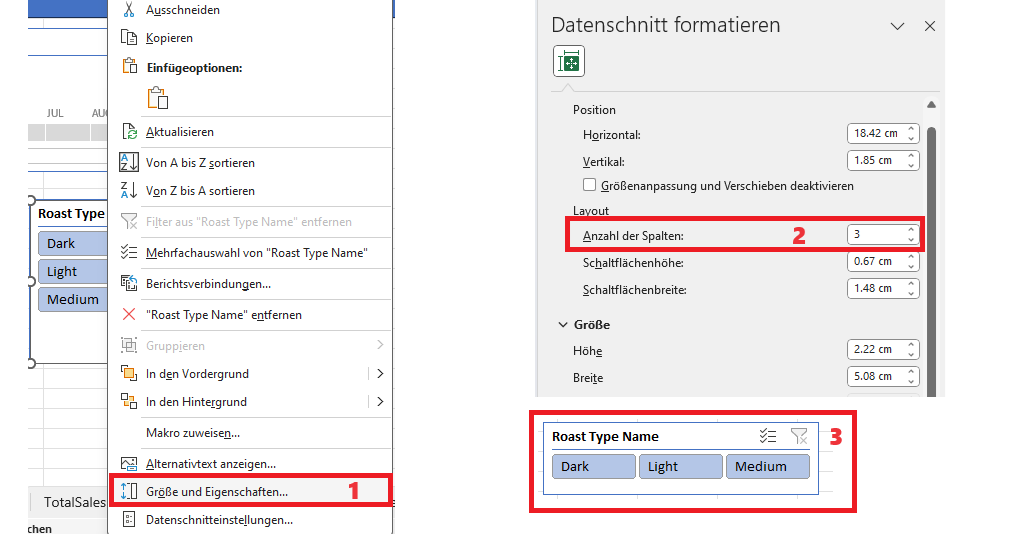
By default the Slicer object is initially created with 1 column. It can be formatted by selecting Slicer's right-click menu option Größe und Eigenschaften (1) and enter the column count in the field Anzahl der Spalten (2) and the Slicer will be transformed to show data in defined number of columns (3)
0.5-Building interactive Dashboard
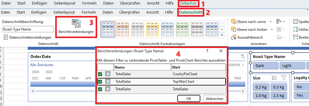
All Dashboard components are created and the last step is connect Slicer and Timeline objects to visuals (4). To connect Timeline or Slicer to visuals there is a button Berichtsverbindungen (3). Depending which object is selected, the button is either under Zeitachse menu option (1) or Datenschnitt menu option (2)
To align all the objects it's used Holding Alt button in order the shape to be automatically snap to grid. The Dashboard is finished, and it will be used to answer the business questions.
1-Total sales by country in 2021 breakdown by Roast type
2-Top month in year 2019 for each coffee type
3-Breakdown by pack size and find top 5 customers overall
4-For Ireland find the most popular Roast type year-wise
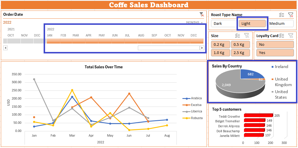
5-Top 5 customers in 2022 with/without a Loyalty card