Barry on Data Analysis

Data Analysis BLOG - description

This blog is created by Barry The Analyst, data analyst, software developer & owner of this web site. The articles contain description of various data analysis platform features with many practical examples. Main Home blog page contains following article types: Data Analysis in general, Excel, SQL/DB, Power BI, Python, JavaScript and Playwright. There are also Portfolio projects that demonstrates Data Analysis features with real Datasets. Gadgets on the right side contain article index (archive) grouped by article type, as well as some additional notes on different topics related to data analysis & software development

The page Portfolio contains portfolio projects on real Datasets using tools & technologies described in articles of this blog.

1. Data Analyst at 47 - to be or not to be? (May)
2. Core Excel functions for Data Analysis (June)
3. Database fundamentals (July)
4. Built-in data structures in Python (August)
5. LOOKUP function family (September)
6. SQL essential features (October)
7. Branching, loops & functions (November)
8. Data Analysis roles & goals (December)

Full stack App deployment with containerization

Sunday, 06.04.2025

To install specified package and add it to 'dependencies' section in package.json it is commonly used npm install e.g. npm install mssql. This can be accomplished with npm install --save as well, which is default behavious. To install and save dependecy into devDependecies of package.json it is used npm install --save-dev

npm install mssql
npm install --save mssql // default
npm install --save-dev mssql
npm install -D mssql // shorthand

NoSQL Database overview

Sunday, 09.03.2025

NoSQL databases started gaining widespread acceptance around the mid-to-late 2000s, with their growth really accelerating during the 2010s. The term "NoSQL" was first coined by Carl Strozzi in 1998 for a relational database that didn’t use SQL, but the term didn't really take off until the mid-2000s. The rise of web applications with high traffic and the need for scalability beyond traditional relational databases (RDBMS) highlighted the limitations of SQL-based systems, particularly with horizontal scaling (across multiple machines). The inspiration for many NoSQL databases was Google's Bigtable paper published 2007, outlining a distributed storage system designed to scale horizontally.

Mainstream Adoption started on 2012 - The term NoSQL became widely recognized, and the technology started being used in production systems for major companies like Facebook, Twitter, Netflix, and LinkedIn.

By the late 2010s, NoSQL databases were considered standard solutions for specific use cases:

High-availability systems (e.g., MongoDB, Cassandra)

Real-time applications (e.g., Redis, Apache HBase)

Big Data and Analytics (e.g., Hadoop ecosystem, Elasticsearch)

Social media, gaming, and IoT applications (e.g., Neo4j for graph databases, Redis for caching)

Today, many organizations use NoSQL in hybrid architectures alongside traditional relational databases, selecting the best database for each use case. Key Factors Contributing to Widespread Acceptance:

Scalability: NoSQL databases were optimized for horizontal scaling, making them better suited for applications that needed to scale out to handle high traffic and large datasets.

Flexibility: The schema-less nature of NoSQL allowed developers to store and retrieve complex and changing data without rigid schemas.

Big Data and Cloud: The rise of cloud computing and big data technologies like Hadoop and Spark further fueled the adoption of NoSQL databases, as they could easily handle large volumes of semi-structured and unstructured data.

Developer Demand: With the explosion of web applications, mobile apps, social media, and IoT devices, developers needed databases that were flexible, high-performing, and scalable.

Document-type NoSQL Databases

Data is stored as documents (usually in JSON or BSON format). Documents are grouped into collections. Each document contains fields, which can be key-value pairs, arrays, or nested objects. Schema-less (documents can have different structures). Suitable for loosely connected or independent data but not optimized for complex relationships. Primarily used for document retrieval via key lookups or more advanced queries based on fields.

Use cases of Document-type DB
- You need flexible schemas.
- Your data has complex, nested relationships.
- You perform frequent read queries on specific fields.
- Your data is relatively independent and doesn’t have complex relationships

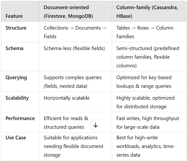
Column-family type NoSQL Databases

Data is stored in tables with rows and columns, but unlike relational databases Columns are grouped into column families, Each row can have a variable number of columns and Data is retrieved by row keys. Optimized for high-speed writes and distributed data.

Use cases of Column-family DB
- You handle large-scale, high-write operations (e.g., logs, time-series).
- You need fast retrieval with predictable access patterns.
- You work with distributed databases requiring high availability.

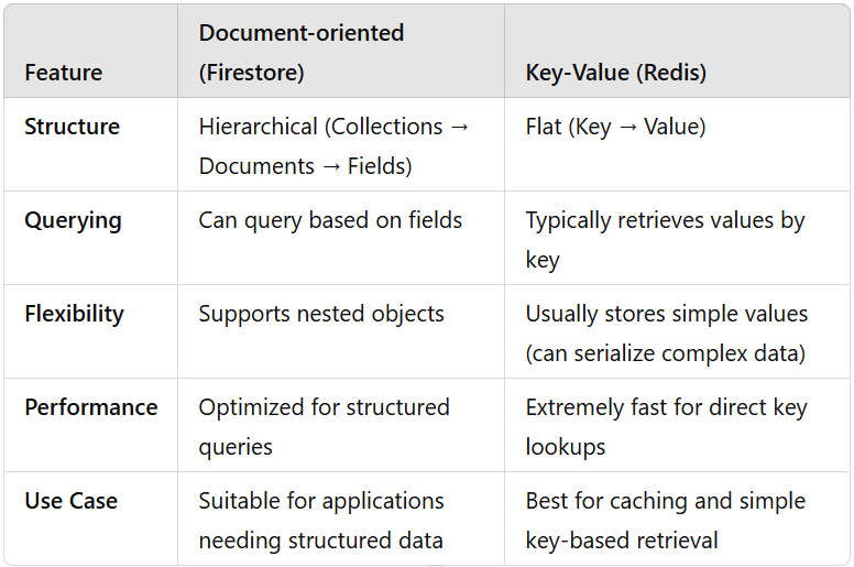
Key-value type NoSQL Databases

Data is stored as a simple key-value pair. Keys are unique identifiers. Values can be strings, lists, sets, or even entire serialized objects. No hierarchy like collections and documents.

Use cases of Key-value DB
- You need ultra-fast reads and writes for simple key-based lookups (e.g., caching, session storage).
- Your data is mostly independent and doesn’t require complex queries or relationships.
- You require high scalability for applications handling millions of read/write operations per second.
- Your use case involves real-time processing, such as leaderboards, API rate limiting, or IoT sensor data.
- You need temporary storage with auto-expiry, like feature flags, shopping carts, or ephemeral sessions.

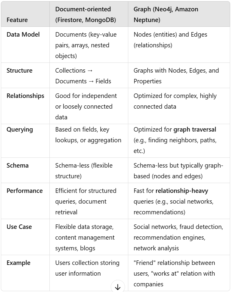
Graph-type NoSQL Databases

Data is represented as nodes (entities), edges (relationships between entities), and properties (information about nodes or edges). Highly optimized for storing and traversing relationships. Nodes are linked by edges. Schema-less but typically follows a graph structure with nodes and relationships. Highly optimized for traversing and querying relationships (e.g., finding shortest paths, recommendations, etc.). Efficient querying of complex, interconnected data through graph traversal (e.g., using Cypher in Neo4j).

Use cases of Graph DB
- Your application involves complex relationships and you need to frequently traverse these relationships (e.g., recommendations, social networks, or fraud detection).
- You need to efficiently query the connections between entities and find patterns (e.g., shortest path, connected components).
- Your data’s value comes from its interconnectedness rather than individual data points.

JavaScript in Test Automation and beyond

Sunday, 16.02.2025

A test runner with Jest-like assertions @playwright/test is developed and maintained by the Playwright team that is built on top of the Playwright API. This test runner is tightly integrated with Playwright and is specifically designed for end-to-end testing. It has capabilities like browser-specific tests, parallel test execution, rich browser context options, snapshot testing, automatic retries and many more.

There are two ways of handling new page opened in child window (using link with target="_blank"):

const [newPage] = await Promise.all(
  [ context.waitForEvent('page'),//page is Event name
    docLink.click(), ] )

const pagePromise = context.waitForEvent('page'); //no await!
await docLink.click();
const newPage = await pagePromise;

In order to create a button in HTML and provide interaction using JavaScript there are following steps to be implemented:

<head> 
<script type="text/javascript" src="path/scp.js"></script>
</head> 
<body>
  <button id="btnID">Click me...</button>
</body>

function clickRun() {
    console.log("Thank you for your click!");
}
// Attach event listeners
document.addEventListener("DOMContentLoaded", function () {
  const elementBtn = document.getElementById("btnID");
  elementBtn.addEventListener("click", clickRun);
});

The first parameter of addEventListener is key of DocumentEventMap interface

The following code performs file upload using File open Dialog:

function loadFile() {
  // Create an invisible file input element
  const fileInput = document.createElement("input");
  fileInput.type = "file";
  fileInput.click(); //(1) Opens the file picker dialog
  // (2) Fired change event ...
  fileInput.addEventListener("change", function () { //(3)
      if (fileInput.files.length > 0) {
          const file =fileInput.files[0];
          console.log("Selected file:", file.name);
          // Read file content
          const reader = new FileReader();
          reader.onload = function (event) { //(6)
            let fileContent = event.target.result;
            console.log("File Content:\n", fileContent);
          };
          reader.readAsText(file); // (4)...(5) Fired onload
      }
  });
}

There is workflow explained:

(1)-The user selects a file

(2)-The change event fires

(3)-The fired change event triggers the event listener

(4)-The FileReader.readAsTextFile() reads the file

(5)-When reading complete, the browser automatically fires the onload event

(6)-The fired onload event triggers reader.onload event handler

It is common and safe practice in JavaScript to define event handlers before triggering events. The consistent event-driven pattern -to define what happens before starting the action- ensures that when the file reading is finished, the handler is attached. If event handler was defined after file reading action, there is a tiny posibility for event to be lost. Is the event-driven pattern consistency ruined by calling fileInput.click() before event listener for change event? The pattern is still intact because the "change" event listener is set up before the event can possibly be fired. There is no race condition since user action is required.

Accumulator pattern

When appending HTML content using innerHTML it has to be used accumulator pattern. Every time innerHTML is set, the HTML has to be parsed, a DOM constructed, and inserted into the document. When writing to the DOM it can be created whole elements only, and they are placed to the DOM at once.

let htmlContent = "openTag";
htmlContent += "elementContent";  
htmlContent += "closeTag";
element.innerHTML += htmlContent;

Function with variable number of parameters

The ...rest syntax collects all remaining arguments into an array

function f(param1, ...rest){
    console.log("rest:", rest);
}
f(1,2,3,4); //Output: rest: [2,3,4]

JavaScript Intermediate (2)

Sunday, 26.01.2025

There are 3 layers of standard web technologies: HTML, CSS and JavaScript. HTML is the markup language that we use to structure to the web content. CSS is a language of style rules that we use to apply styling to the HTML content, to look more beautiful. JavaScript is a scripting language that enables the web page to be interactive.

Use for...in loop to iterate throug JSON object. When applied to array, it will get array index for each element. Using for...of loop wil iterate values in array.

const jsonOb = {"key1" : 111, "key2": 222};
const arrX = ["first", "sec", "third"];
for( let key in jsonOb )
  console.log(key, jsonOb[key]); //key1 111 key2 222  
for( let key in arrX )
  console.log(key); // 0,1,2
for( let value of arrX )
  console.log(value); //first sec third

To connect to MS SQL Server database from Node.js, perform query and run SQL script, the first step is to install mssql. After that import the needed objects setup configuration of database connection:

const sql = require('mssql');
const fs = require('fs');
const path = require('path');
const config = { // Configuration for DB connection
    user: 'sa',
    password: 'myPwd',
    server: 'remote-server', // You can use 'localhost\\instance' to connect to named instance
    database: 'MY_DB',
    options: { encrypt: false, // Use true if your server supports encryption
               trustServerCertificate: true } };// Change to true for local dev / self-signed certs

Connection is established using sql.connect() method, that returns sql.ConnectionPool object. Running query or SQL script is done using pool.request().query():

async function getData() { 
try {
  let pool = await sql.connect(config);
  let res = await pool.request().query(`SELECT * FROM MY_T`);
  const scriptPath = path.join(__dirname, 'script.sql');
  const script = fs.readFileSync(scriptPath, 'utf8');
  res = await pool.request().query(script);
  console.log('Script executed successfully:', res);
  return res.recordset; } 
catch (err) { console.error('SQL error', err); } 
finally { sql.close();} }

await getData().then(data => {
  console.log('Data retrieved:', data);
}).catch(err => { console.error('Data Error:', err); });

For loading data from CSV file and parameterizing query to get file path it is used dynamic SQL. When DB table needs to be either updated or new record inserted, it is used MERGE statement to ensure the right action:

DECLARE @FilePath VARCHAR(255);
SET @FilePath = 'C:\Path\To\File\DataSrc.csv';
DROP TABLE IF EXISTS #tmpTable;
CREATE TABLE #tmpTable(a nvarchar(5) not null, b nvarchar(6) not null);
DECLARE @BulkInsertSQL NVARCHAR(500);
SET @BulkInsertSQL = N'
    BULK INSERT #tmpTable 
    FROM ''' + @FilePath + N''' 
    WITH (
        FIRSTROW = 2, 
        FIELDTERMINATOR = '';'', 
        ROWTERMINATOR = ''\n'', 
        CODEPAGE = ''65001'', -- Specifies UTF-8 encoding
        DATAFILETYPE = ''widechar'' );'; -- Unicode (NVARCHAR)
EXEC sp_executesql @BulkInsertSQL;

MERGE INTO TABLE_DEST AS Dest
USING #tmpTable AS Source
ON Dest.Field1 = Source.Field1s 
WHEN MATCHED THEN
  UPDATE SET Dest.Field2=Source.Field2s, Dest.Field3=Source.Field3s
WHEN NOT MATCHED BY TARGET THEN
  INSERT(ID, Field2, Field3) 
  VALUES(LOWER(NEWID()), Source.Field2s, Source.Field3s);

To generate unique string based on current datetime with granulation of 1 minute and length up to 4 characters for next 14 years and up to 5 characters for next more than 200 years, it is cool to use Base 62:

const BASE62_CHARS = '0123456789ABCDEFGHIJKLMNOPQRSTUVWXYZabcdefghijklmnopqrstuvwxyz';
function toBase62(num) {
  if (num === 0) return '0';
  let str = '';
  while (num > 0) {
      const remainder = num % 62;
      str = BASE62_CHARS[remainder] + str;
      num = Math.floor(num / 62); }
  return str; }

export function generateStrUnique(){
  const datetimenow = new Date();
  const year = datetimenow.getFullYear()-2025;  
  const month = datetimenow.getMonth();
  const day = datetimenow.getDate();
  const hour = datetimenow.getHours();
  const minute = datetimenow.getMinutes();
  let valueNum =  (year << 20) | (month << 16) | (day << 11) | (hour << 6) | minute;                 
  return String(toBase62(valueNum)); }

File system I/O operations: use path.dirname to extract directory path from the file path. To ensure that directory exists and to create new one if it doesn't use fs.mkdirSync. Use fs.existsSync to check if file exists, and fs.unlinkSync to delete it if it does. To append line into the file use fs.appendFileSync and to read file content use fs.readFileSync. In order to completely rewrite the file content, use fs.writeFileSync.

const fs = require('fs');
const path = require('path');
const dirPath = path.dirname(strFilePath);
fs.mkdirSync(dirPath, { recursive: true });
if (fs.existsSync(strFilePath)) 
  fs.unlinkSync(strFilePath);
fs.appendFileSync(strFilePath, htmlContent, 'utf8');
const htmlFile = fs.readFileSync(strFilePath, 'utf-8');
fs.writeFileSync(strFilePath, htmlContent, 'utf-8');

DOM manipulation methods are inherently browser-based and aren't directly available when working with Node.js on the server side. When using fs.readFileSync to read an HTML file into a string variable in Node.js, it's dealing with plain text without a DOM to interact with. To achieve DOM-like manipulation on the server side, there is JSDOM - a popular library that simulates a subset of browser APIs, including the DOM, within Node.js. This allows you to manipulate HTML documents as if you were in a browser environment. In order to update particular HTML section defined by ID the code follows:

const htmlContent = fs.readFileSync(filePath, 'utf-8');
// Initialize JSDOM with the HTML content
const dom = new JSDOM(htmlContent);
// Access the document
const document = dom.window.document;
// Use getElementById to find the target div
const myDiv = document.getElementById(idSection);
myDiv.innerHTML += "New line to add";
// Serialize the updated HTML back to a string
const updatedHTML = dom.serialize();
// Write the updated HTML back to the file 
fs.writeFileSync(filePath, updatedHTML, 'utf-8');

Automated Test Containerization

Sunday, 01.12.2024

Docker is an open platform for developing, shipping, and running applications. Docker enables you to separate your applications from your infrastructure so you can deliver software quickly. With Docker, you can manage your infrastructure in the same ways you manage your applications. By taking advantage of Docker's methodologies for shipping, testing, and deploying code, you can significantly reduce the delay between writing code and running it in production.
Docker provides the ability to package and run an application in a loosely isolated environment called a container. The isolation and security lets you run many containers simultaneously on a given host. Containers are lightweight and contain everything needed to run the application, so you don't need to rely on what's installed on the host. You can share containers while you work, and be sure that everyone you share with gets the same container that works in the same way.

To setup automation test development environment:
------------------------------------------
1. Install VSCode and git
2. Install Node.js: from https://nodejs.org/en. This is essential as Playwright is a Node.js library.
-Add to Path NODE_HOME="C:\Program Files\nodejs"
-To check if it is installed run: npm --version
3. Playwright Framework: Install Playwright using npm
-To check if it is installed run: npx playwright --version
-To check if installed globally run: npm config get prefix and check for Playwright files and/or folders in node_modules
-To clear cache if previous playwright remained: npx clear-npx-cache
-To clear cache from npm: npm cache clean --force
Run: npm init playwright if starting new Playwright project
-Select JavaScript, folder to put end-to-end test
-Select to Install Playwright browsers or manually via "npx playwright install"
-This command initializes a new Playwright testing project in the current directory
-It creates all the necessary configuration files and sets up the folder structure for Playwright tests
-It installs @playwright/test and other necessary dependencies
-It creates playwright.config.js (configuration for the Playwright project) and example tests in the tests folder
-It keeps environment clean - all dependencies are installed locally (not globally) keeping the project isolated
3-A If you already have a Node.js project and just want to add Playwright for testing, use npm install @playwright/test
4. Create the first test
-In PowerShell create new spec.js file:
New-Item -Path ./tests -Name "first-test.spec.js" -ItemType "File"
-Skeleton of the first-test.spec.js file is as follows:

const { test, expect } = require('@playwright/test');

test('Navigate to a webpage', async ({ browser }) => {
  // Create a new browser context and page
  const context = await browser.newContext();
  const page = await context.newPage();
  // Navigate to your desired URL
  await page.goto('https://www.google.com');
  // Keep the browser open for 3 seconds (optional)
  await page.waitForTimeout(3000);
  // Close the context
  await context.close();
});

5. Select browser to use, for Edge ensure there is only the following item in the projects array within playwright.config.js:

/* Configure projects for major browsers */
projects: [ { name: 'Microsoft Edge',
  use: { ...devices['Desktop Edge'], channel: 'msedge'}, }, ],

6. Create folder for JS files, create first module and Hello World function. In order to call this function from spec file, it has to be exported from JS file and imported in spec file

// module01.js
function helloWorld() {
    console.log("Hello world!"); }
module.exports = { helloWorld };

// first-test.spec.js
const { helloWorld } = require('../utils/module01');

7. Run the test using command
npx playwright test first-test.spec.js --headed
-In PowerShell if it doesn't execute, run the following
Set-ExecutionPolicy RemoteSigned -Scope Process

To containerize project using Docker:
------------------------------------------
1. Install Docker Desktop
-Ensure Docker is installed: docker --version
2. Add Dockerfile to project root and test locally:
-Create a Docker image by running: docker build -t my-app-name .
-Run Docker image by command: docker run --rm my-app-name
-Run interactively by: docker run -it my-app-name /bin/bash

3. Add Dockerfile to root project folder
-This file describes how to package your app into a container. This setup ensures your app runs entirely within the container, independent of the host machine.
FROM command:
-When using the Playwright Docker image (mcr.microsoft.com/playwright), the necessary browsers are preinstalled in the container and there is no need to install them manually
RUN command:
-There is no need to add a separate installation step for Playwright in the Dockerfile, if the devDependencies in the package.json include @playwright/test, which is Playwright's official testing library. As long as @playwright/test is listed in package.json, npm install ensures Playwright is installed in the container
-When RUN npm install executes, it will install all the dependencies listed in the devDependencies section of the package.json, including Playwright.

# Use Playwright's official Docker image with browsers FROM mcr.microsoft.com/playwright:v1.36.0-focal # Set working directory in the container WORKDIR /app # Copy project files into the container COPY . . # Install project dependencies RUN npm install # Expose a port if needed (optional, for web-based apps) # EXPOSE 3000 # Default command to run all tests (or runtime user-defined) CMD ["npx", "playwright", "test"] # Default command to run specific test script #CMD ["npm", "run", "create-item"]

4. Add a docker-compose.yml in the root of your project, to simplify running the container.

version: '3.8' services: playwright-app: build: context: . image: playwright-app container_name: my-playwright-container volumes: - .:/app stdin_open: true tty: true

5. Test locally: docker compose up --build

To setup automation test PRODUCTION environment:
------------------------------------------
1. Node.js: This is essential as Playwright is a Node.js library.
To check if it is installed run: npm --version
2. Playwright Framework: They need to install Playwright using npm.
To check if it is installed run: npx playwright --version
3. Your Code: Provide all the necessary scripts and files.
4. VSCode (Optional): If they need to edit or debug the code.
5. Run: npm init playwright
6. Run: npm install playwright
7. Run: npm install @playwright/test
8. Configure Playwright: Set up the Playwright configuration file.
9. Run Tests: Use the appropriate npm scripts to execute the tests.
Besides a.m. core dependencies, if your project uses additional libraries or tools, make sure to include them in your package.json file.

6. Client step 1 Install Docker Desktop on their Windows machine

7. Client step 2 Obtain your Docker image
You have two options:
7.1. Share the Docker image:
---Push it to Docker Hub or another registry:
docker tag playwright-app your-dockerhub-username/playwright-app
docker push your-dockerhub-username/playwright-app
---Client can pull it:
docker pull your-dockerhub-username/playwright-app
docker run --rm your-dockerhub-username/playwright-app
7.2. Share your project folder:
---Your client can clone/download it, then run:
docker compose up --build

8. Client step 3 Simplify running the app:
---Create a Shortcut: Use a .bat file for Windows to run the container with a click:
@echo off
docker compose up --build
pause
Save this file as run-tests.bat in the project folder

#run ALL tests: docker run my-playwright-container #run SPECIFIC test: docker run my-playwright-container npx playwright test CreateItem.spec docker run my-playwright-container npm run switch-item

JavaScript Intermediate

Sunday, 04.11.2024

There are 3 layers of standard web technologies: HTML, CSS and JavaScript. HTML is the markup language that we use to structure to the web content. CSS is a language of style rules that we use to apply styling to the HTML content, to look more beautiful. JavaScript is a scripting language that enables the web page to be interactive.

Iterating through array using forEach. If need to use break, it's better to use regular for loop.

let arrTest = [1,2,4];
arrTest.forEach(function(element,index){ //can take 2 params
      console.log(element, index)   });

arrTest.forEach((el,index) => { console.log(el, index) });

A shorter way to write function is Arrow function. It is easier to read, but does not enable hoisting as regular functions do, which stands for possibilty to call a function before it's definition.

const regularFunction = function () { console.log('Rf'); }
const arrowFunction = () => { console.log('Af'); }

If Arrow function has only 1 parameter, parentheses are not needed

const oneParam = (param) => { console.log(param+1); };
const oneParam = param => { console.log(param+1); };
oneParam(2); // output writes 3

If Arrow function has only 1 line, return and {} are not needed

const oneLine = () => { return 2 + 3; };
const oneLine = () => 2 + 3;
console.log(oneLine()); // output writes 5

Built-in function setTimeout is a practical example of callback function which means passing a function to another function as parameter.

setTimeout(function() {
  console.log("function called in the future") }, 3000); 
console.log("asyncronously line after but called first");

// Implementing delay
await new Promise((resolve) => setTimeout(resolve, 5000));

Built-in function setInterval runs periodically. There is example with running it each 1s within interval of 5s

let isRunning = false;
let hasToRun = false; // initially on page load
let intervalId;
function resetInterval() {
  hasToRun = !hasToRun;
  if (hasToRun && !isRunning) {
      intervalId = setInterval(function () {  // Start 
          console.log("Running interval ...");
      }, 1000);
      isRunning = true;
  } else if (!hasToRun && isRunning) { // Stop the interval
      clearInterval(intervalId);
      isRunning = false; }
}

resetInterval(); // Toggle on
await new Promise(resolve => setTimeout(resolve, 5000)); 
resetInterval(); // Toggle off

To get time interval between 2 Date objects in proper format:

function getDuration( dtStart, dtEnd ) {
  const ms = dtEnd - dtStart;
  const seconds = Math.floor(ms / 1000);
  const minutes = Math.floor(ms / (1000 * 60) );
  const hours = Math.floor(ms / (1000 * 60 * 60));
  let duration = String(ms % 1000) + 'ms';
  if( seconds > 0 )
      duration = (String(seconds % 60)) + 's ' + duration;
  if( minutes > 0 )
      duration = (String(minutes % 60)) + 'min ' + duration;
  if( hours > 0 )
      duration = (String(hours)) + 'h' + duration; 
  return duration; } // 1h 23min 33s 129ms

To update value for particular key in JSON file:

updateJSONfile(key, value)
{
  const fs = require('fs');
  const filePath = './path/file.json';
  try {
      // Read the existing file
      const fileContent = fs.readFileSync(filePath, 'utf-8');
      const data = JSON.parse(fileContent);
      data[key] = value; // Modify the data
      fs.writeFileSync(filePath, // Write updated data back 
              JSON.stringify(data, null, 2), 'utf-8');
  } catch (err) {
      console.error('[***Error handling JSON file]', err);
  }
}

JavaScript Basics (2)

Sunday, 06.10.2024

There are 3 layers of standard web technologies: HTML, CSS and JavaScript. HTML is the markup language that we use to structure to the web content. CSS is a language of style rules that we use to apply styling to the HTML content, to look more beautiful. JavaScript is a scripting language that enables the web page to be interactive.

Truthy and falsy values are supersets of true and false. String can be defined with '-' or "-" or backticks `-` (template strings) which is the most flexible option, that allows to pass variable and to create multiline string as well. There are 3 shortcuts for if statement:

Ternary operator

Guard operator && resolves the first expression and if falsy the second expression doesn't get resolved.

Default operator || sets the default value as the second expression so if the first value truthy the second expression doesn't get resolved

if( !value ) //check for false, 0, '', NaN, undefined, null
let a = 5 
const str = `The Number that is defined in the variable
            is five=${a}`; // Inserts 5, multiline string
const res = (a === 6 ? truthy : falsy) //Ternary operator
const b = (a != falsy) && a * 2 //Guard operator
const c = (a / 0) || 'Cannot resolve' //Default operator

If accessed the object's property that doesn't exist it will return undefined value. To delete propery use function delete obj.property.

Object property can be function as well, that can be defined by using shorthand method as well.

const product = { 
      calc: function calcPrice() { return 100; } };

const product = { calc() { return 100; } }; //Shorthand method

const price = product.calc();

Using destructuring as a shortcut to assign object's property to the variable of the same name. If property and variable have the same name, by creating an object can be used shorthand property shortcut

const message = objectPostman.message;
const { message } = objectPostman; // Destructuring 
const { message, post } = objectPostman; // More as well
const objectPost2 = { message }; // Shorthand property

TheJSON built-in object can convert JS object to string and vice versa.

const strJSON = JSON.stringify(product);
product = JSON.parse(strJSON);

Using localStorage built-in object to save and load state between browser refresh. It will survive Ctrl+F5, but after clearing cookies from browser setting it will reset value

let visits = localStorage.getItem('visits') || '0'
visits = Number(visits); //Convert to number
visits++;
localStorage.setItem('visits', visits);
alert(visits);
localStorage.removeItem('visits'); //removing item

The DOM built-in object is the objects that models (represents) the web page. It combines JS and HTML together and provides with full control of the web within JavaScript. The method querySelector() lets us get any element of the page and put it inside JS, returning the first one if there are more. If element is found, it return JS object (accessing value returns string), otherwise it returns null. Unlike innerHTML, innerText will trim inner text. For input element it is used value property.

document.body.innerHTML = 'New content';
document.title = 'New title';
document.querySelector('button') //<button>Caption</button>
document.querySelector('button').innerHTML //Caption
document.querySelector('button').innerHTML='New'//New
document.querySelector('button').innerText // Trim
str = document.querySelector('input').value // <input>
num = Number(str) //convert to do math operations
str = String(num) //converts number to string

To dynamically set image, passed as variable imageName:

const element = document.querySelector('img');
element.innerHTML = `<img src="images/${imageName}.png>`

To access class list and modify class content in JS:

const btn = document.querySelector('button');
btn.classList.add('new-class');
btn.classList.remove('not-needed-class');

The window built-in object represents the browser.

window.document // DOM root object
window.console // built-in console objects
window.alert // popup

Object event and event listeners are used for event handling

onclick=click

onkeydown=key press

onscroll=scrolling

onmouseenter=hovering over

onmouseleave=stop hovering over

Using property key of the object event can be ckech if particular key pressed

<input onkeydown="if(event.key === 'Enter') handleEnter();
  else handleOtherEvents(event);"

Playwright Test Automation with JavaScript (3)

Sunday, 01.09.2024

A test runner with Jest-like assertions @playwright/test is developed and maintained by the Playwright team that is built on top of the Playwright API. This test runner is tightly integrated with Playwright and is specifically designed for end-to-end testing. It has capabilities like browser-specific tests, parallel test execution, rich browser context options, snapshot testing, automatic retries and many more.

To setup automation test environment:
------------------------------------------
1. Node.js: This is essential as Playwright is a Node.js library.
2. Playwright Framework: They need to install Playwright using npm.
3. Your Code: Provide all the necessary scripts and files.
4. VSCode (Optional): If they need to edit or debug the code.
5. Run: npm init playwright
6. Run: npm install playwright
7. Run: npm install @playwright/test
8. Configure Playwright: Set up the Playwright configuration file.
9. Run Tests: Use the appropriate npm scripts to execute the tests.
Besides a.m. core dependencies, if your project uses additional libraries or tools, make sure to include them in your package.json file.

To compare locators, their handles have to be evaluated and compared:

const handle1 = await loc.elementHandle();
const allHandles = await collLocs.elementHandles();
for (let i = 0; i < allHandles.length; i++) {
    const handle = allHandles[i];
    // Pass both handles wrapped in an object to eval
    const isSame = await loc.page().evaluate(
        ({ el1, el2 }) => el1 === el2, 
        { el1: handle1, el2: handle }  ); }

Split string by defined delimiter returns string array

let arrURL = server.split('//'); // https://site.com
let strProtocol = arrURL[0] // gets "https:"

Waiting for locator to be visible using state (timeout is optional) or assertion. In particular, assertion to be 1 locator exactly

loc.waitFor({ state: 'visible', timeout: 5000 });
await expect(loc).toBeVisible();
await expect(loc).toHaveCount(1);

Locator returned from locator() method on page or other locator (DOM subtree search) will be valid object, if not found it will be locator that points to nothing with count() == 0, and locator.nth(n) will not raise an error if n is out of range

To wait for an element to be updated on the page with new value:

const selT = 'p.class1';
// Poll every 500ms to log the text content        
for (let i = 0; i < 20; i++) {  // timeout = 10 s
    const currentDisplay = await this.page.textContent(selT);
    if( currentDisplay == "Expected" ) //text updated
        break;
    await this.page.waitForTimeout(500); } // Wait

To wait for a page with specific URL and check it

page.waitForFunction(() => window.location.href.includes('S'));
page.url().includes('PartOfURL')

Traversing the DOM tree

Accessing parent element is possible for one or more levels

locParent = locChild.locator("..")
locGranpa = locChild.locator("../..")

Get the next sibling and list of all following siblings

locNextSib = locChild.locator('xpath=following-sibling::*[1]')
locAllFlwSibs = locChild.locator('xpath=following-sibling::*')

Checking if root node is reached while searching level-up

const tg = await loc.evaluate(el => el.tagName.toLowerCase());
if (tg === 'html')

Playwright Reporting

To implement custom report using CustomReporter class:

// custom-reporter.js
class CustomReporter {
  async  renameReportFile(oldPath, newPath) {
    const fs = require('fs').promises;
    try {
        await fs.rename(oldPath, newPath);
        console.log(`Renamed from ${oldPath} to ${newPath}`);
    } catch (error) {
        console.error(`Error file: ${error.message}`); }
  }  
  async onEnd(result) {
    console.log('Updating Report file name...');      
    await this.renameReportFile("old/index.html", newPath());
    console.log(`Status: ${result.status}`);
    console.log(`Started at: ${result.startTime}`);
    console.log(`Ended at: ${result.endTime}`);
    console.log(`Total duration: ${result.duration}ms`);
  }     
}  
module.exports = CustomReporter;

// playwright.config.js
module.exports = defineConfig({ ... reporter: [
    ['html', { outputFolder: 'test-results', open: 'never' }],
    ['./tests/custom-reporter.js'] ],

Playwright Test Automation with JavaScript (2)

Sunday, 25.08.2024

Playwright provides a set of APIs that allow developers and testers to write test scripts to automate web applications across different browsers, such as Chromium, Firefox, and WebKit. It supports multiple programming languages like Java, TypeScript, Python, C# and of course - JavaScript. To setup environment, the first step is to install Node.js - an open-source, cross-platform, back-end JavaScript runtime environment that runs on the V8 engine and executes JavaScript code outside a web browser.

Install Node.js

Add to Path NODE_HOME="C:\Program Files\nodejs"

Install VSCode

Run: npm init playwright

Run: Set-ExecutionPolicy RemoteSigned -Scope Process

The command npm init playwright installs Playwright locally. It installs @playwright/test package (the Playwright test library) into your project's node_modules directory as a local dependency. The Playwright CLI is available within the project scope but not system-wide. To check Playwright version it shoud be run npx playwright --version

To wait until particular element is visible, or if it is attached to the DOM:

await locator.waitFor({ state: 'visible'})
await locator.waitFor({ state: 'attached'})

After option in combo box is selected, or datetime from Datetimepicker connected to input element is chosen, current content (selected option or datetime) is extracted using inputValue method.

Methods toHaveValue() and inputValue() are appropriate for input fields, as their text is stored in the value attribute. This method works for <input>, <textarea> and <select> elements, directly giving value attribute of the selected option

locInput = await page.locator('input#ID') 
extractedValue = locInput.inputValue();
await expect(extractedValue).toContain('textToContain')
await expect(locInput).toHaveValue('textToContain')

Method toContainText() is designed for verifying text within elements like labels, divs, spans or other non-input elements where text is part of the DOM content (innerText or textContent).

locLabel = await page.locator('label#ID2') 
await expect(locLabel).toContainText('textToContain')

The methods page.locator can return one, many or none locators. To ensure it found element tried to locate it can be used count() method. If it returns many locators, it cannot be iterated through as an array, but using particular locator methods:

locElements = await page.locator('#ID') 
locElements.count() !=0 //ensure returned at least 1 locator
//if returned many, loop through array of locators this way:
const n = await locElements.count();
for(let i=0; i<n; i++)
  await itemText = locElements.nth(i).textContent();

To locate an element by its text content using exact or partial match:

page.locator('tag.class:text("Partial match")')
page.locator('tag.class:text-is("Exact match")')

To check if an element contains particular class

//Extracting the value of the 'class' attribute
classAttValue = locElement.getAttribute('class')
classAttValue.includes('required-class')

To locate element by its class and text content using XPATH

sel = 'xpath=//span[contains(@class,"c1") and text()="Abc"]'
locElement = page.locator(sel);

Searching for particular text on the page using backticks, scroll page up and down using keyboard, log array as table using console.table and highlighting particular element

page.locator(`text="${strTextToFind}"`)
await page.keyboard.press("PageDown")
console.table(arrToShow)
locator.highlight()

Global login - Re-use state & Re-use Authentication

There are 3 main actions that have to be performed on browser, context and page objects.

saving current state in JSON file

injecting this state on creating new context

navigating page to URL where login process started (not final URL after logging in is done!)

await context.storageState({path: 'LoginAuth.json'})

c2 =await browser.newContext({storageState: 'LoginAuth.json'})
page = await c2.newPage();
await page.goto("https://site.domain.com/LoginStartPage");

STEP 1 - the first step is to create Global setup file, containing globalSetup() function which will run once before all tests. There will be authentication code in that file and using Playwright storage state capability the state of application after logging in will be stored. The function has to be exported to be used from test function.

//global-setup.js
async function globalSetup(){
  const browser = await chromium.launch({headless: false,
    executablePath: 'C:\\Program Files (x86)\\Microsoft\\Edge\\Application\\msedge.exe'
  });
  const context = await browser.newContext();
  const page = await context.newPage();
  await doLogin(); //login code
  //Save the state of the web page - we are logged in
  await context.storageState({path: "./LoginAuth.json"});
  await browser.close(); //cleanup
}
export default globalSetup;

STEP 2 - update playwright.config.js to use global-setup file, this line is to be added to the level of timeout parameter

globalSetup: "./global-setup",

STEP 3 - in order to use stored state that we have logged into, it needs to be added line in use section of playwright.config.js.

storageState: "./LoginAuth.json",

STEP 4 - in order to re-use stored state from JSON file in client code remove the line from config file and load stored settings from JSON file in the client code

//storageState: "./LoginAuth.json",

c2 =await browser.newContext({storageState: 'LoginAuth.json'})
page = await c2.newPage();
await page.goto("https://site.domain.com/LoginStartPage");

STEP 5 - some particular test can be configured either to use specified JSON file other that defined in config (before function implementation), or to clear cookies and perform login action (inside function body)

test.use({ storageState: "./ParticularAuth.json"}); //Option 1
test("Pw test", async ({ page, context })){
  await context.clearCookies(); //Option 2 - clearing cookies

JavaScript Basics (1)

Sunday, 28.07.2024

There are 3 layers of standard web technologies: HTML, CSS and JavaScript. HTML is the markup language that we use to structure and give meaning to our web content, for example defining paragraphs, headings, and data tables, or embedding images and videos in the page. CSS is a language of style rules that we use to apply styling to our HTML content, for example setting background colors and fonts, and laying out our content in multiple columns. JavaScript is a scripting language that enables you to create dynamically updating content, control multimedia, animate images, and many other things.

Declaring variable or constant and get its type:

var a = 5 
let b = 6
const c = 7
console.log(typeof(a))

Declaring array, access its elements:

var marks = Array(4) //4 elements, empty 
var marks = new Array(6,7,8,9) //one way
var marks = [6,7,8,9] //another way
console.log(marks[0]) //access 1st element - Returns 6

Iterating array elements:

let i = 0; 
for(let element of marks)
  console.log("Element Nr. ", i++, "=", element)

Append, delete, insert, get index of particular element, check presence of particular element:

marks.push(10) //Added to end 10 [6,7,8,9,10] 
marks.pop() //Deleted last [6,7,8,9]
marks.unshift(5) //Insert in the beginning [5,6,7,8,9]
marks.indexOf(7) //Returns 2 - index of 7
marks.includes(99) //Returns false - 99 not present in Array

Slice includes first index, excludes last index. Length,

subArr = marks.slice(2,4) //Returns [7,8]
marks.length //Returns 5 = array length

Reduce, filter and map.

//Anonymous function, 0 is initial value, marks[5,6,7,8,9]
let total=marks.reduce((sum,mark)=>sum+mark,0) //Returns 35 
let evens=marks.filter(element=>element%2==0) //Returns [6,8]
let dbl=marks.map(element=>element*2) //Rets. [10,12,14,16,18]

Sorting an array

arr.sort() //for string array ASC
arr.reverse() //Reversing an array
arr.sort((a,b)=>a-b) //number array ASC
arr.sort((a,b)=>b-a) //number array DESC

Class declaration, exporting and importing

class MyClass
{
  constructor(property_value)
  {
    this.my_propery = property_value;
  }
}
module.exports = {MyClass}

const {MyClass} = require('./path/to/class')

Global variable declaration, exporting and importing

export let x1 = dataSet.sys;

import { x1 } from '../path/declared.js';

Creating and calling asynchronous test function

test('First Playwright test', async({ browser }) => {
  const context = await browser.newContext();
  const page = await context.newPage();
  await page.goto("www.google.com");
});

Iterating through JavaScript object (key-value pair collection)
Use for...of for arrays when you want the values

const keysOfObject = Object.keys(object1)
for(let key of keysOfObject)
   const itemValue = object1[key]

Use for...in for objects when you need the property names (keys)

for (let key in object1) {
  const itemValue = object1[key] }

Working with Date object

const date1 = new Date() //current datetime
let date2 = date1; //by ref =>pointer
let date3 = new Date(date1) //by value =>copy
let date4 = new Date(2024,11,5,10,25); //11=Dec, 0-based month
date1.toISOString(); //shorter string

The Math.floor() static method always rounds down and returns the largest integer less than or equal to a given number. Math.round() rounds number, and Math.random() generates random number between 0 and 1;

const a = 4.5
let b = Math.floor(a) //b=4
let c = Math.round(a) //c=5
let r = Math.random() //between 0 and 1

Playwright Test Automation with JavaScript (1)

Sunday, 23.06.2024

Playwright provides a set of APIs that allow developers and testers to write test scripts to automate web applications across different browsers, such as Chromium, Firefox, and WebKit. It supports multiple programming languages like Java, TypeScript, Python, C# and of course - JavaScript. To setup environment, first is to be installed node.js and after that to perform the following steps:

Add to Path NODE_HOME="C:\Program Files\nodejs"

Install VSCode

Run: npm init playwright.

Run: Set-ExecutionPolicy RemoteSigned -Scope Process

Selecting page object using CSS selector by ID, class, attribute and text:

Locator = page.locator('#ID') 
Locator = page.locator('tag#ID')
Locator = page.locator('.classname') 
Locator = page.locator('tag.classname')
Locator = page.locator("[attrib='value']")
Locator = page.locator("[attrib*='value']") //using RegEx
Locator = page.locator(':text("Partial")')
Locator = page.locator(':text-is("Full text")')

This will return element, on which will be perfomed actions - fill(), click() etc.

Extracting text present in the element (grab text). How long will Playwright wait for element to come to DOM is defined in config file, { timeout = 30 * 1000 }

const txtExtracted = Locator.textContent()

The following is defined in the config file:

const config = {
  testDir: './tests', //run all tests in this dir
  timeout: 30 * 1000, //timeout for each test
  expect: {
    timeout: 5000 //timeout for each assertion
  },

Assertion - check if defined text is present in element (->Doc: Assertions). How long - defined in config file { expect: { timeout: 5000 } ...}

expect(Locator.toContainText('Part of text'))

Traverse from parent to child element - Parent element has class parentclass, and child element has tag b

<div abc class="parentclass" ...
    <b xyz ...
page.locator('.parentclass b')

When returned list of elements (->Doc: Auto-waiting) - Playwright will wait until locator is attached to the DOM, few ways to access particular list element.
It can also be extracted text present in all returned locators and assigned to array, but Playwright won't wait until locators are attached to the DOM:

LocatorsList = page.locator('.class1') //more elements
LocatorsList.nth(0)
LocatorsList.first()
LocatorsList.last()
const arrReturnedElementsText = LocatorsList.allTextContents()
//returns [el1, el2, el3]

To wait until locators are attached to DOM (->Doc: waitForLoadState) it is required to add an additional synchronization step

//Option 1 - (discouraged)
await page.waitForLoadState('networkidle')
//Option 2
LocatorsList.first().waitFor()

Handling static DDL, Radio button, Check box

const ddl = page.locator("select.classname") //Locate DDL
await ddl.selectOption("OptionValuePartOfText") //select opt.
const rb1 = page.locator(".rbc").first() //1st RB option
await rb1.click()
await expect(rb1.toBeChecked()) //assertion
await rb1.isChecked() //returns bool value
await cb1.click()
await expect(cb1.toBeChecked())
await cb1.uncheck()
expect( await cb1.isChecked() ).toBeFalsy() //action inside

Opening Playwright Inspector to see UI actions

await page.pause()

Check if there is particular attribute and value

await expect(Locator).toHaveAttribute("att","val1")

Child windows handling with Promise. There are 3 stages of Promise: pending, rejected, fulfilled.

const newPage = await Promise.all([
    context.waitForEvent('page'),
    docLink.click(),
])

Pytest & Playwright Web Automation Testing

Sunday, 19.05.2024

Pytest is a popular Python testing framework that offers a simple and flexible way to write and run tests. Playwright is a modern, fast and reliable browser automation tool from Microsoft that enables testing and automation across all modern browsers including Chromium, Firefox and Webkit. In this article series, there will be shown how to blend Playwright capabilities into the Pytest framework with the use of pytest-playwright plugin.

Python features covered in this article
---------------------------------------------
-BrowserType.launch(headless, slowmo)
-Browser.new_page()
-Page.goto()
-Page.get_by_role('link', name)
-Locator.click()
-Page.url
-Browser.close()
-Page.get_by_label()
-Page.get_by_placeholder()
-Page.get_by_text()
-Page.get_by_alt_text()
-Page.get_by_title()
-Page.locator - CSS selectors, Xpath locators
-Locator.filter(has_text)
-Locator.filter(has)

Getting started - Environment setup

Checking Python version, creating and activating virtual environment, installing Playwright, updating pip, checking playwright version:

First it will be checked if Python is installed using python --version

After that it will be created virtual environment to keep things clean, using python -m venv venv

Virtual environment will be activated using .\venv\Scripts\activate

To install Playwright inside of virtual environment it will be used pip install playwright command

If noticed to update, pip will be updated with command python.exe -m pip install --upgrade pip

Checking Playwright version will be done using playwright --version command

To download and install browser drivers Playwright needs in order to run test scripts it will be used playwright install command

PS C:\Users\User\PyTestPW> python --version
Python 3.11.2
PS C:\Users\User\PyTestPW> python -m venv venv
PS C:\Users\User\PyTestPW> .\venv\Scripts\activate
(venv) PS C:\Users\User\PyTestPW>
(venv) PS C:\Users\User\PyTestPW> pip install playwright
Successfully installed greenlet-3.0.3 playwright-1.44.0 pyee-11.1.0 typing-extensions-4.11.0
[notice] A new release of pip available: 22.3.1 -> 24.0
(venv) PS C:\Users\User\PyTestPW> python.exe -m pip install --upgrade pip
Successfully installed pip-24.0
(venv) PS C:\Users\User\PyTestPW> playwright --version
Version 1.44.0
(venv) PS C:\Users\User\PyTestPW> playwright install  
Downloading Chromium 125.0.6422.26 ... 100%
Downloading Firefox 125.0.1 ... 100% 
Downloading Webkit 17.4 ... 100%

Creating simple test script

The first script consists of the following steps:

Launching the browser

Opening new page

Visiting Playwright Python website

Clicking on the link - Docs menu item

Printing URL of the clicked link

The following code is implemented in new file app.py :

# FILE: app.py
from playwright.sync_api import sync_playwright

with sync_playwright() as playwright:
    # Select Chromiun as browser type on Playwright object
    bws_type=playwright.chromium    
    # Launch a browser using BrowserType object
    browser = bws_type.launch()
    #Create a new page using Browser object
    page = browser.new_page()
    #Visit the Playwright website using Page object
    page.goto("https://playwright.dev/python/")
    #Locate a link element with "Docs" text
    docs_btn=page.get_by_role('link', name="Docs")
    #Clink on link using Locator object
    docs_btn.click()
    #Get the URL from Page object
    print("Docs: ", page.url)
    #Closing method on Browser object
    browser.close()

By default headless argument in the launch method is True (no UI shown), and by setting it to False the browser UI will be shown. To see the script execution in slow motion it can be used slowmo argument (slowmo=500 means 500 times slower execution) in the same launch method of the BrowserType object

To locate link to be clicked, in inspection mode when positioning mouse on the link there will be shown HTML section of the particular element:
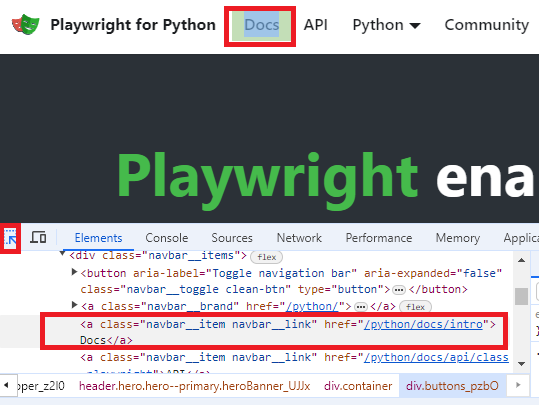
Link is located using get_by_role() method of page object, and clicked using click() method of the returned object.

Running our script from Terminal:

(venv) PS C:\Users\User\PyTestPW> python app.py
Docs:  https://playwright.dev/python/docs/intro

Selecting Web elements in Playwright

In the Method get_by_role() the first argument is object type - link, button, heading, radio, checkbox..., and the 2nd argument is the object name. Method is called on Page object and returned value is Locator object

Method get_by_label() can be used for input field that has a label element associated, as in example below

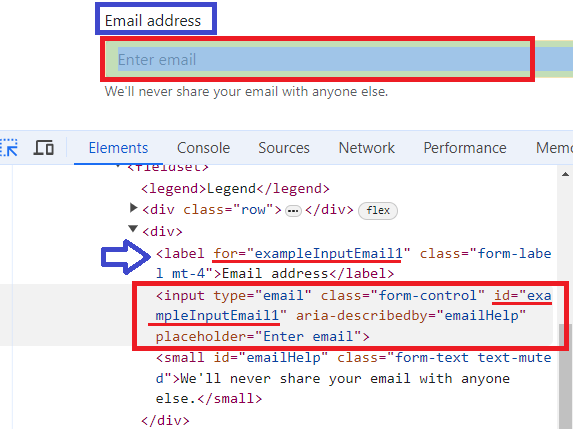
If input field has no label associated, it can be located using get_by_placeholder() method. Locating element using inner text locator (caption of the button, paragraph containing searched text, etc...) is done using method get_by_text(). Locating image by alt text is done using get_by_alt_text() method. For elements that have title attribute specified and unique, it can be used get_by_title() method for locating the element.
All of the a.m. methods return Locator object.

CSS selectors

Locating a web element using CSS selector is done using Page.locator method (passing "css=" is optional). When locating using tag name, it is done by passing it as the first argument, locating using class name class is separated from tag name by dot and locating using id it is separated from tag name by hash. Lastly, locating using attribute is done using tag name and square bracket notation, and if an attribute has a value assigned the value is included within square brackets.

page.locator("css=h1") #Tag
page.locator("button.btn_class") #class
page.locator("button#btn_id") #id
page.locator("input[readonly]") #attribute
page.locator("input[value='val1']") #att with value

Web element can be also located using CSS pseudo class. Locating by text pseudo class matching text is loose, and for the strict match it is used text-is pseudo class selector. To locate element that is visible it is used visible pseudo class. To select element based on its position it is used nth-match pseudo class selector.

page.locator("h1:text('Nav')") # loose selection
page.locator("h1:text-is('Nav')") # strict selection
page.locator("div.dropdown-menu:visible")
page.locator(":nth-match(button.btn-primary, 4)")

Xpath Locators

Using XML querying language specifically created to select web elements is one more way to locate elements on the web page (passing "xpath=" is optional). Absolute path starts with slash(/) and relative path starts with double slash (//). It can be selected object based on attribute and value as well. Using Xpath functions provides more flexibility. Exact match of the text inside of element is located using text() function, and loose match is done using contains() function. That function can be used for other attributes as well, such as class.

page.locator("xpath=/html/head/title") # Absolute path
page.locator("//h1") # Relative path
page.locator("//h1[@id='navbars']") # Attribute and value
page.locator("//h1[ text()='Heading 1']") # Exact match
page.locator("//h1[ contains(text(), 'Head')]") # Loose match
page.locator("//button[ contains(@class, 'btn-class1')]") # class attribute

Other locators

If there are more elements of the same type with the same name, it is used locator(nth) function and passed 0-based index of the particular element we want to locate. This function can be appended to CSS selector as well, since it also returns locator object. To locate parent element it used double-dot (..). Selecting element by id or by its visibility can be also accomplished using locator method. Using filter() method it can be selected element either based on its inner text with has_text argument or based on containment of another element with has argument

page.get_by_role("button", name="Primary").locator("nth=0")
page.locator("button").locator("nth=5") 
page.get_by_label("Email address").locator("..") # Parent
page.locator("id=btnGroupDrop1") # id
page.locator("div.ddmenu").locator("visible=true") # visible
page.get_by_role("heading").filter(has_text="Heading")
parent_loc = page.locator("div.form-group") # containment
parent_loc.filter(has=page.get_by_label("Password"))

Playwright basic features

Sunday, 07.04.2024

Test automation has become significant in Software Development Life Cycle (SDLC) with the rising adoption of test automation in Agile teams. As the scope increases, new tools for test automation are emerging in the market. Test automation frameworks are a set of rules and corresponding tools that are used for building test cases, designed to help engineering functions work more efficiently. The general rules for automation frameworks include coding standards that you can avoid manually entering, test data handling techniques and benefits, accessible storage for the derived test data results, object repositories, and additional information that might be utilized to run the tests suitably.

Playwright is a powerful testing tool that provides reliable end-to-end testing and cross browser testing for modern web applications. Built by Microsoft, Playwright is a Node.js library that, with a single API, automates modern rendering engines including Chromium family (Chrome, MS Edge, Opera), Firefox, and WebKit. These APIs can be used by developers writing JavaScript code to create new browser pages, navigate to URLs and then interact with elements on a page. In addition, since Microsoft Edge is built on the open-source Chromium web platform, Playwright can also automate Microsoft Edge. Playwright launches a headless browser by default. The command line is the only way to use a headless browser, as it does not display a UI. Playwright also supports running full Microsoft Edge (with UI).

Playwright supports multiple languages that share the same underlying implementation.
-JavaScript / TypeScript
-Python
-Java
-C# / .NET
All core features for automating the browser are supported in all languages, while testing ecosystem integration is different.

Playwright is supported on multiple platforms: Windows, WSL, Linux, MacOS, Electron (experimental), Mobile Web (Chrome for Android, Mobile Safari). Since its release in Jan 2020 Playwright has a steady increase in usage and popularity.

Playwright is Open Source - it comes with Apache 2.0 License, so all the features are free for commercial use and free to modify.

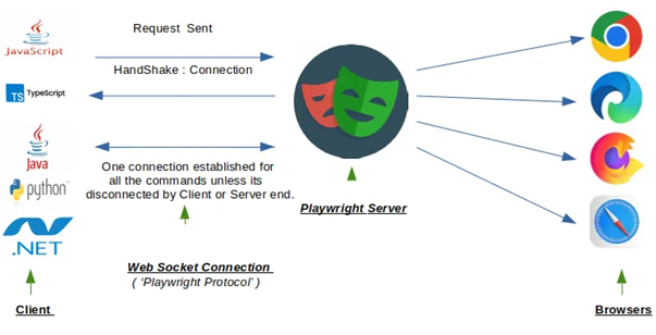
Architecture Design (Communication)

Playwright uses ChromeDevTool (CDP) – WebSocket protocol to communicate with the Chrome browser’s rendering engine. WebSocket is a stateful protocol.

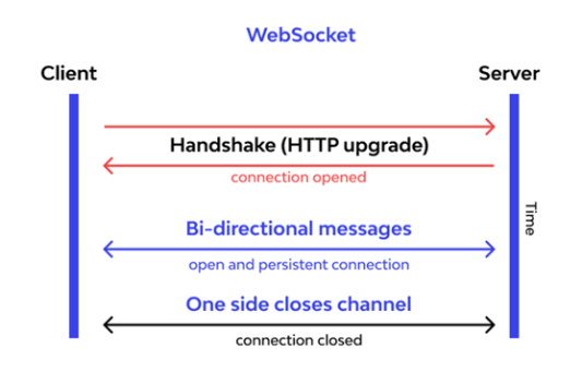
Playwright will communicate all requests through a single web socket connection that remains active until all tests have been completed. This design might reduce points of failure during test execution and makes Playwright a more stable, speedy test execution and reduces flakiness.

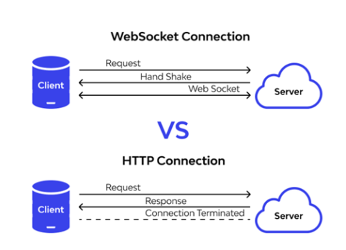
Since Playwright protocol works on web socket connection, it means once the request is sent from the client end, there is a handshake connection established between client and playwright server. That is a single connection that stays open between code ( the commands written like click , fill , select ) and the browser itself. This connection remains open throughout the testing session. It can be closed by the client and server itself.

Further Benefits of using Playwright

Easy Setup and Configuration - Being a Test Automation Framework, it just needs a configuration as the installation doesn’t take much time. Depending on the language we use with Playwright, the installation steps might change

Types of Testing: Playwright supports Functional, End to End, and API Testing. With a third-party plugin, Playwright can be integrated with Accessibility Testing.

Locator strategy: Playwright supports various locator types: id, class, CSSSelector, XPath, Angular/Vue/React component, accessibility attributes, etc. and has ability to filter locators, chain multiple locators together, locate elements by their relative layout, to define your own selector by customizing the default selector engine

Parallel Browser Testing: Playwright also supports the execution of simultaneous tests (AKA parallel testing) through Browser Context and can run parallel tests with multiple browsers. This scales up testing and comes in handy when multiple web pages must be tested simultaneously.

Support for Multiple Tab/Browser Window: Playwright supports multi-tab and multi-window. Some test cases must verify the scenario by launching a new window and returning to the parent window. Playwright supports all different types of test cases.

Test Isolation: Each test in Playwright is executed in a unique browser context. A browser context is equivalent to a browser’s incognito-like profiles. This means that each context has its own local storage, session storage, cookies, etc. This delivers full test isolation with zero overhead. They are fast and cheap to instantiate.

Built-in Reporters: Playwright framework, by default, comes with many valuable reporters like List, Dot, Line, JSON, JUnit, and HTML Reporters. The exciting part is that with Playwright, one can create custom reporters. Playwright also supports third-party reporter Allure Report.

Typescript Support out of the box: Zero configuration is required for typescript language support as it understands your typescript and javascript code.

CI/CD Integration Support: Playwright supports CI/CD integration. It even provides docker images for some language bindings.

Debugging Tools Support: Playwright testing supports different debugging options making it developer-friendly. Some debugging options are Playwright Inspector, VSCode Debugger, Browser Developer Tools, and Trace Viewers Console Logs.

Lambda functions and map()

Sunday, 24.03.2024

Function map() allows us to map a function to a python iterable such as a list or tuple. Function passed can be built-in or user-defined, and since it is not a function calling, just passing an adress, it's to be used a function name with no parenthesis(). Lambda function is an anonymous function defined in one line of code, and it is especially suitable for using in map() function. The code from all examples is stored on GitHub Repository in Jupiter Notebook format (.ipynb).

Python features covered in this article
---------------------------------------------
-map()
-list() for conversion to list
-lambda function
-get() function on dictionary
-tuple() for conversion to tuple

Function map()

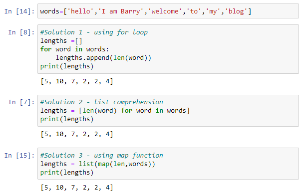
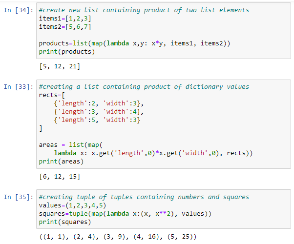
Map function helps us to be more explicit and intentional in code. Map function takes as arguments a function and an iterable on which elements passed function will be performed. It returns map object which can be converted to list using list() function or to tuple using tuple() function, as well as to many other types or classes. There are 3 examples that shows using map() function compared to other possible solutions in creating a new list that contains length of elements in the list:

Using lambda function in map

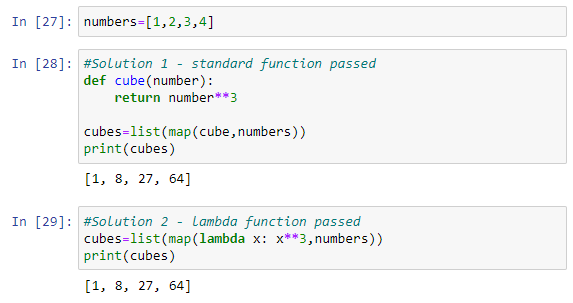
Using lambda function is a practical way for defining a map function, because it requires less lines of code and reduces dependency (user-defined function has to be defined previously if using a standard way). There are 2 examples illustratiing both ways, function passed to map() calculates cube of each list element:

Applying map() to many lists, a dictionary and tuple

We can pass more iterables to map() functions, for instance two lists and define with a lambda function an operation to be performed on elements of each one. List can contatin dictionary elements, which can be safely accessed using get() function and passing 0 for the case that an element doesn't exist. Lambda function passed to map() function can return tuple as well. There are examples:

Creating Pivot tables in Python

Sunday, 25.02.2024

Pivot tables known from Excel (also known as Matrix tables from Power BI) can be created in Python as well. A pivot table is a powerful data analysis tool that allows us to summarize and aggregate data based on different dimensions. In Python, pivot tables can be created using the pandas library, which provides flexible and efficient tools for data manipulation and analysis.

Python features covered in this article
---------------------------------------------
-pivot_table()
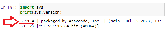
-sys.version
-pivot_table(values)
-pivot_table(agg_func)
-pivot_table(columns)
-pivot_table(fill_value)
-pivot_table(margins)
-pivot_table(margins_name)

DataSet in Excel is downloaded from GitHub and using head() function there are top 5 records shown.

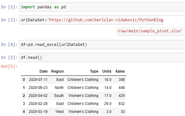
The code used in this article is available as Jupiter Notebook on GitHub repository

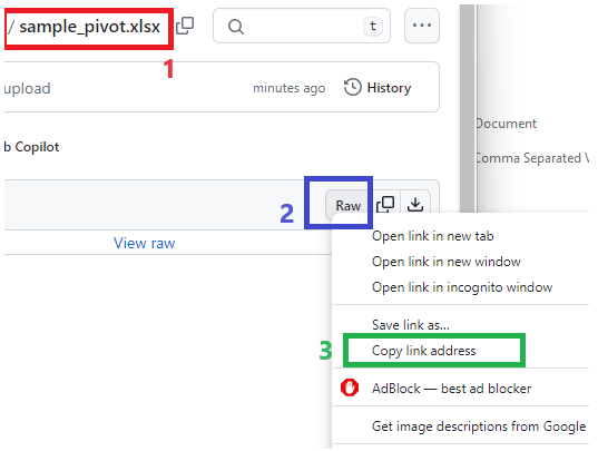
To ensure obtaining the right URL path from GitHub it has to be used Raw option. First click on the file(1) then on the Raw option(2) from the Right-Click menu select Copy link address option(3)

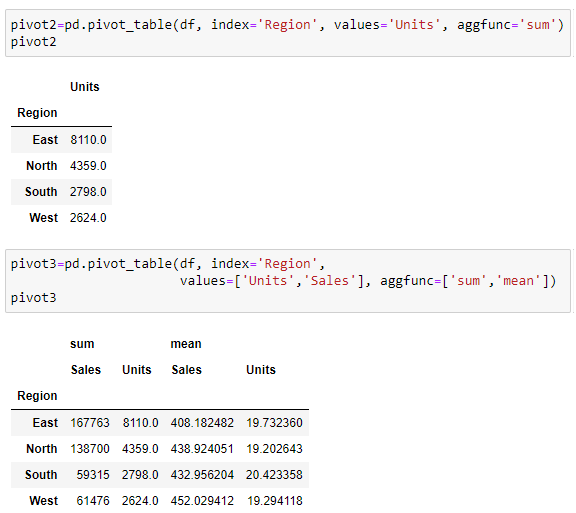
Let's create Pivot table using pivot_table() function that will show values of the columns Sales and Units with applied some aggregating function. There will be explicitly passed names of columns to be aggregated

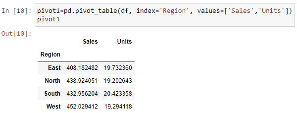
Values shown in the table above are average (mean) values because 'mean' is the default aggregating operation in pivot_table() function.

In previous versions of pandas there were automatically selected numerical columns that could be aggregated and dropped columns contatining other data types (strings, datetime...) for which it made no sense to aggregate. However, in the current version

it is still possible, but there is a warning that in future version it will not be possible anymore:

If we want to calculate another aggregate function, for instance sum function we can pass it as an agg_func argument to pivot_table function. Aggregating columns can be one or more, as well as aggregating functions:

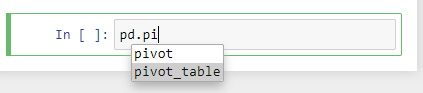
To use autocomplete feature in Jupiter Notebook, it should be pressed TAB after dot:

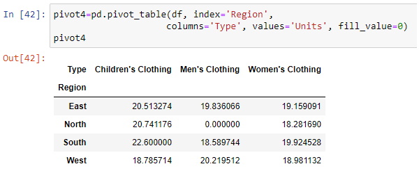
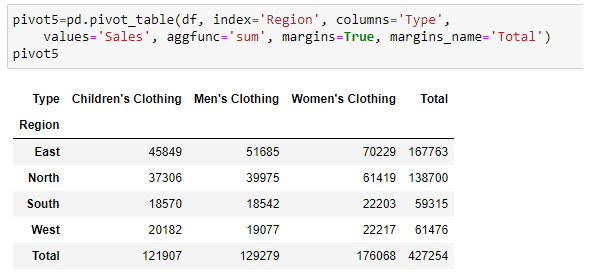
Breaking out data by region and also by type of sales in columns can be done using columns argument of pivot_table function. By using fill_value argument it can be filled empty cells in the DataFrame with specified values.

Showing totals can be done using margins argument of pivot_table function. Using margins_name it can be defined name of total column and row:

Exploring pandas Series

Sunday, 28.01.2024

In Data Anaysis process the Data exploration refers to the initial step, in which data analyst uses available feature of the tool or programming language to describe dataset characterizations, such as size, quantity, and accuracy, in order to better understand the nature of the data. Exploring data is just the first look, looking at it if it's going to be cleaned up doing the data cleaning process. Then it's going to be done the actual data analysis actually finding trends and patterns and then visualizing it in some way to find some kind of meaning or insight or value from that data. The code used in this article is available on GitHub repository

Python features covered in this article
-----------------------------------------------
-DataFrame.dtypes
-Series.describe()
-Series.value_counts(normalize)
-Series.unique
-Series.nunique()
-crosstab
-%matplotlib inline
-Series.plot
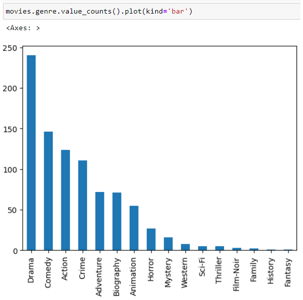
-Series.value_counts().plot()

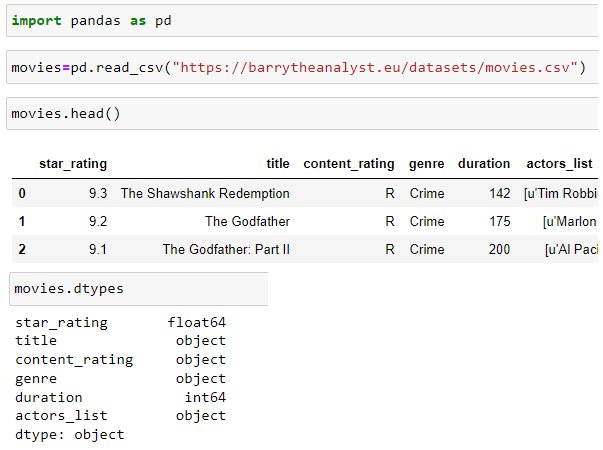
The data set that will be explored in this article is IMDB movies rating data set, that is available on GitHub repository It will be loaded to DataFrame object and using DataFrame.dtypes first it will be explored column data types:

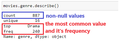
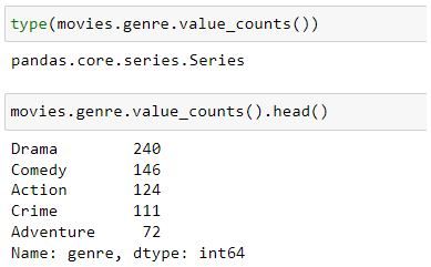
Exploring column [genre] can be started with method Series.describe() that will show some information about Series (column):

More detailed information will be shown using method Series.value_counts() with optional use of normalize parameter which will show percentages

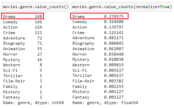
Type of object that value_counts() method returns is also Series, so all Series methods are available, for instance head():

Using Series.unique() method there will be shown all uninque column values, and Series.nunique() method will return number of unique values.

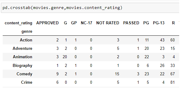
It can be performed cross-tabulation of the two different Series using crosstab() method. This will show one Series as column and another as rows and table will be filled with number of matching pairs - in this case showing how many genre has particular rating

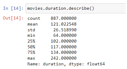
Method Series.describe() can also be applied to numeric column, and in that case it shows some statistics about it:

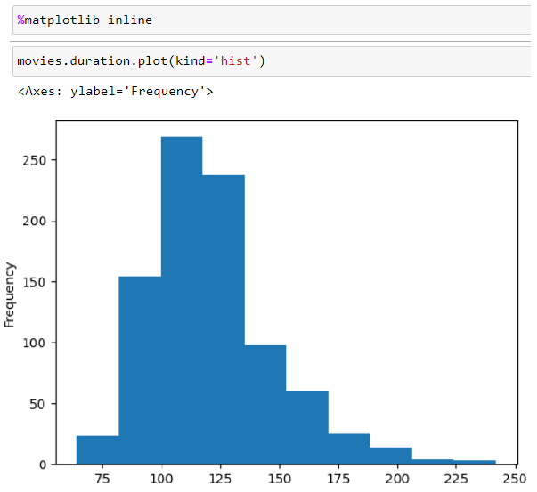
Data Visualization can be shown within Jupiter Notebook using %matplotlib inline command. the following example shows histogram of duration Series, that shows distribution of numerical variable:

The last example shows bar chart of value_counts() applied to Series genre:

Is Data Analysis a Dying Career?

Sunday, 02.12.2023

Besides technical hard skills, a Data Analyst has to have also communication and social soft skills. This is important not only for the job - as the presentation of insights to stakeholders is its regular part - but also for communication about their job. As I seriously intend to be fully engaged as a professional in Data Analysis and stay into it long-term, I shared my plans a few days ago in a small talk with one colleague. He isn't in Data Business but the first thing he asked me is: Does it have a future, since AI can nowadays do so much of the tasks? Well, I told him that AI can help us a lot to be more efficient, more punctual and more productive. But that small conversation motivated me to research a little bit, asking myself: am I going to end up in a dead-end street? Starting to check some relevant facts & figures brought me back in 2012: Harvard Business Review (source: hbr.org) called The Data Science "the sexiest job in 21st century". It has been a hot topic for a decade, now the question is: Is Data Science dying?
NOTE: Terms "Data Scientist" and "Data Analyst" are commonly used interchangeably as well as in this article

Some people think (source: teamblind.com) that Data Science is no longer the sexiest career but it's becoming the most depressing career, since many companies are laying off Data Scientists becoming waste of money for them, and that the field is dying very fast. On the other had, there are headlines from 2022 (source: fortune.com) suggesting a different point of view:

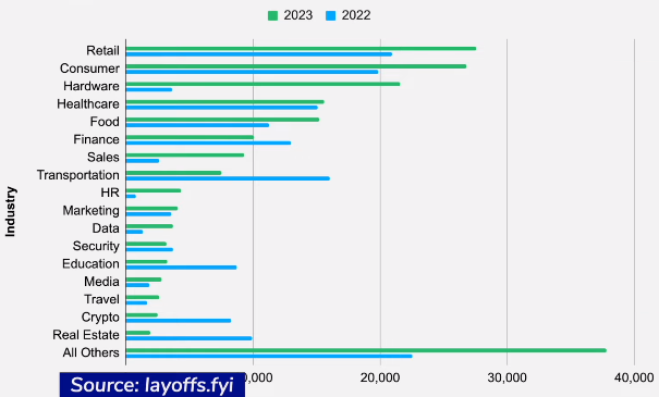
So why are so many people worried about job security in data science? In this worry coming out of nowhere? With recent news about coming layoffs it's natural to be concerned. Comparing 2023 with 2022 accross many industries there are more layoffs in the current year in the most of them (source: layoffs.fyi):

Comparing to other technical roles (source: warntracker.com) layoffs of Data Scientists in Meta and Google are relatively rare, less than 5% in years 2022 and 2023. So, the data indicates that the perception of data scientists facing higher job loss risks doesn't align with reality, since Data Scientists have a relatively lower risk of layoffs compared to other roles considering the current trends in major tech companies.

Some Data Scientist reported (source: teamblind.com) that while others say the field is dying their own career keeps getting better, they keep earning more money and getting promoted. They firmly believe that Data Science is not shrinking but actually growing. They think that many companies still haven't figured out how to use data science effectively. Additionally they observe continuing trend of companies investing in data-driven products indicating that the demand for data science remains strong. Consequently they view data science as extremely relevant and highly sought-after career

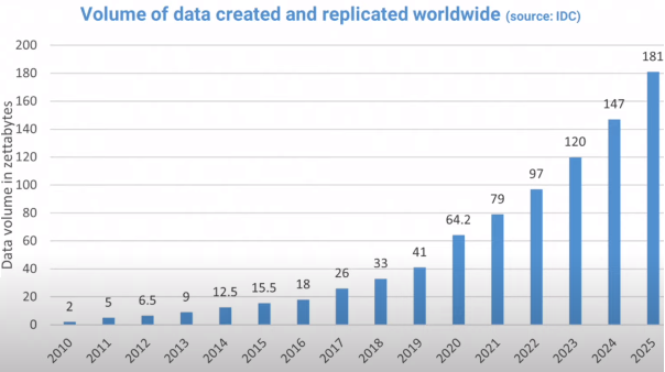
According to one study (source: statista.com) the amount of data in the world is expecting to reach 181 zettabytes by 2025 (1 zettabyte=10^21 bytes):

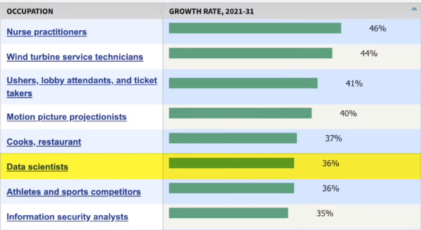
This tremendous growth has led to a high demand for data scientists and it even surpasses the rate at which colleagues and universities can train them. Information obtained from the U.S. Bureau of Labor Statistics (source: bls.gov) show that the number of jobs for data scientists is projected to increase by 36% from 2021 to 2031. making it one of the fastest growing occupations in the U.S:

The number of job opportunities for data scientists has increased significantly in recent years. Since 2016 there has been a staggering 480% growth in job openings for this occupation (source: fortune.com). Job postings on "indeed", a popular job search platform, have also seen since 2013 a notable rise of 256% percent (source: hiringlab.org). Also it is projected (source:bls.gov) that an average of 13,500 job openings for data scientists will be available each year over the next decade as a current workforce retires and it needs to be replaced.

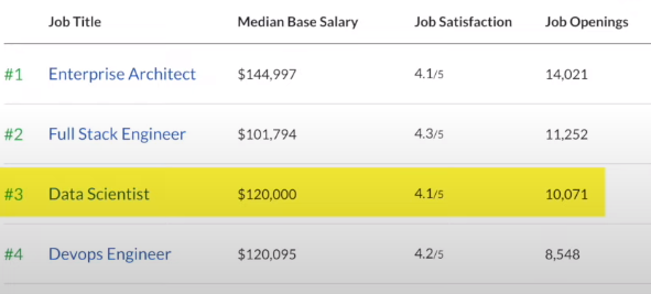
These figures highlight the strong demand for data scientists in the job market. In fact according to Glassdoor's list of the best jobs for 2022, Data Scientist is ranked as the third best occupation in the U.S. surpassing only by Enterprise Architects and Full Stack Engineer:

Considering the supply side of the story - workforce - many people are eager to enter this domain. In the recent announcement from the University of California at Berkeley (source: berkeley.edu) they are creating a new college for the first time in over 50 years. This new College of Computing, Data Science, and Society (CDSS) is born out of the growing demand for computing and data science skills.

Succeeding in Data Science is not only about technical proficiency. It's equally important to have a genuine passion for uncover insights from data, the curiosity to ask the right questions and the creativity to effectively communicate the findings in a manner that others can understand. Strong communication skills are highly valued in this field, as well as nurturing curiosity and being open to exploring new areas within Data Science.

Specifying rules using CONSTRAINTs

Sunday, 12.11.2023

Foreign key is the field in the table which contains values from another table's primary key field. Foreign key is one of the available constraints in table definition and it enforces database integrity. There is also DEFAULT constraint - which will fill the field with specified value if not provided in INSERT INTO statement (if NULL value provided explicitly it will be inserted, not default value). There is CHECK constraint that returns boolean value - TRUE or FALSE, for NULL value it returns UNKNOWN.

SQL features covered in this article
---------------------------------------------
-FOREIGN KEY
-SELECT INTO
-DEFAULT CONSTRAINT
-CASCADING CONSTRAINT
-CHECK CONSTRAINT

There are 2 tables in the database:

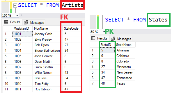
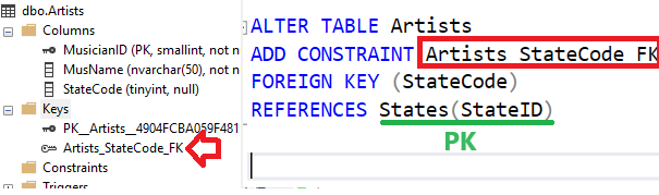
Adding FOREIGN KEY constraint will disable entering records in Artist table with value of the field State that are not in the PK field in State table:

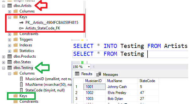
Copy table Artist to a new table for testing can be done using SELECT INTO statement. It wil copy data only, and neither PK nor FK constraints:

Create DEFAULT constraint will fill value if not provided. If provided NULL, field will be filled with NULL value, not the default value.

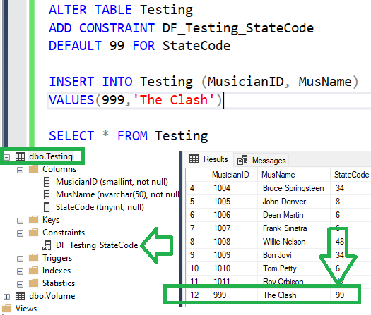
To remain DB referential integrity, there are few options to be defined on the FK. These options define the behaviour of the orphan records in the FK table when PK table record is modified (deleted or updated). Default is 'No action' - meaning PK record cannot be modified. Other options are 'Set NULL/Default' - fill orphan record values with NULL/Default value (defined with DEFAULT constraint) and Cascade - delete all orphan records in FK table when PK table record modified.

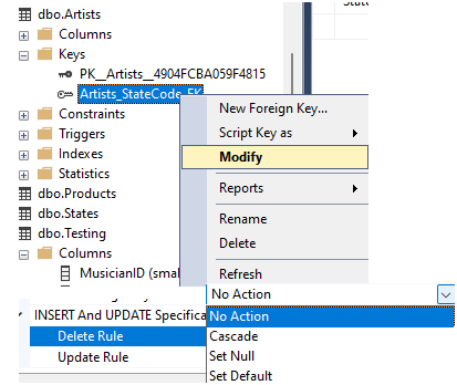
Finally, CHECK constraint limits the value range that can be entered for a column, by defining boolean expression record has to meet:

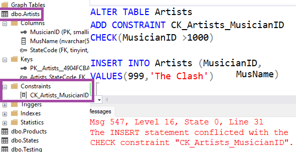
R1C1 notation & German Z1S1 conversion map

Sunday, 22.10.2023

There is a standard cell notation in Excel known as A1 notation i.e. column is referenced as letter and a row is referenced as number. R1C1 is another type of reference style that can be used, in which there are both rows and columns referenced as numbers. In the R1C1 style, Excel indicates the absolute location of a cell with an "R" followed by a row number and a "C" followed by a column number, so R1C1 would refer to the cell in the first row and first column. Similarly, R2C3 would refer to the cell in the second row and third column. It can also be indicated the relative location of the cell using square bracket notation, for instance 3 columns left and 1 row down would be reference to as R[1]C[-3].

Let's see where notation can be set. By default it is set A1 notation. Depending on Excel version the window can look slightly different, cell reference notation is to be set on the
check box in Excel Options->Formulas:

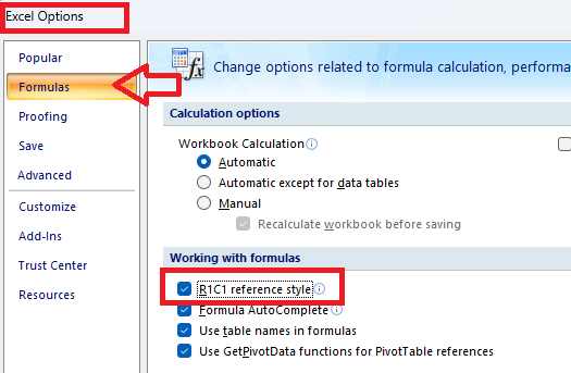
Relative referencing in R1C1 notation is done using square bracket notation. Whether to reference the n cell-distance with positive[n] or negative[-n] number is pretty intuitive - just follow the direction of column and row names:

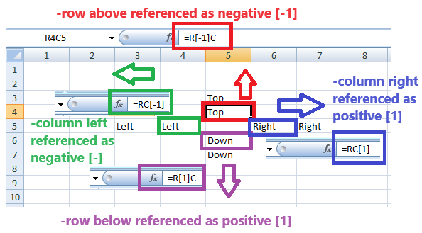
There is an example of simple formula applied in the same column and using relative row reference:

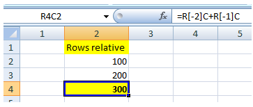
In the next example simple formula applied in the same row and used for relative column reference:

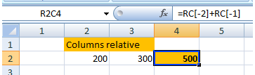
Using absolute reference in R1C1 cell notation (in A1 notation this would be accomplished using dollar ($) symbol), formula can be copied to any other location and it will remain the same, referencing the same cells:

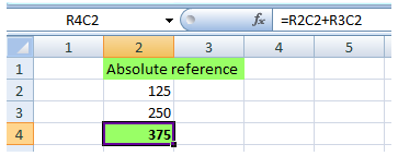
it can also be used mixed referencing when we want to fix row reference and remain a relative column reference (or vice versa). In the following example, the formulas for the cells R5C3 and R5C4 are exactly the same!

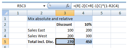
German function conversion map

Besides different name of R1C1 notation - in German it is Z1S1, Z stands for 'Zeile' that means row and S stand for 'Spalte' that means column - there are German names for the other Excel functions as well. There is a table with function map from original English to German, of the functions that are relevant for Data Analisys:

English function	German function
R1C1	Z1S1
IF	WENN
LOOKUP	VERWEIS
VLOOKUP	SVERWEIS
HLOOKUP	WVERWEIS
XLOOKUP	XVERWEIS
SUM	SUMME
SUMIF	SUMMEWENN
COUNTIF	ZÄHLENWENN
AVERAGEIF	MITTELWERTWENN
MAXIFS	MAXWENNS
MINIFS	MINWENNS
MATCH	VERGLEICH
CONCATENATE	VERKETTEN
LEFT	LINKS
RIGHT	RECHTS
MID	TEIL
SUBSTITUTE	WECHSELN
LEN	LÄNGE
TRIM	GLÄTTEN
UPPER	GROSS
LOWER	KLEIN
PROPER	GROSS2
INDIRECT	INDIREKT
COUNT	ANZAHL
COUNTA	ANZAHL2
DAYS	TAGE
NETWORKDAYS	NETTOARBEITSTAGE
ISOWEEKNUM	ISOKALENDERWOCHE
IFERROR	WENNFEHLER
IFNA	WENNNV

Filtering, sorting & indexing data

Sunday, 17.09.2023

Data filtering and sorting can be used together or independently. While sorting organizes the data according to a certain parameter and order (ascending or descending), filtering removes unimportand data from view. Filtering excludes anything not falling within the categories selected (sets a hard boundary) and sorting (setting a soft boundary) changes only the sequence of appearance. Both sorting and filtering are very important when looking at complex datasets or search results.

Python features covered in this article
---------------------------------------------
-DataFrame.isin()
-DataFrame.str.contains()
-DataFrame.set_index()
-DataFrame.filter(items, like)
-DataFrame.loc[]
-DataFrame.iloc[]
-DataFrame.sort_values()
-read_csv(index_col)
-reset_index()
-inplace parameter
-sort_index()
-DataFrame.columns

Dataset will be loaded from CSV file using read_csv() function:

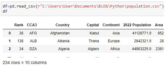
All code used in this article is available on GitHub repository.

Data filtering

Using square bracket operator we can filter data, in this case only to first 4 countries by popuation:

To filter by particular column with specified values defined in a list, it will be used isin() function:

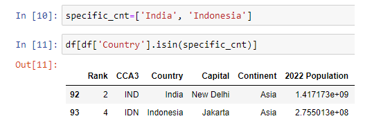
Similar as LIKE operator in SQL, we can use string function contains() to search for specific value:

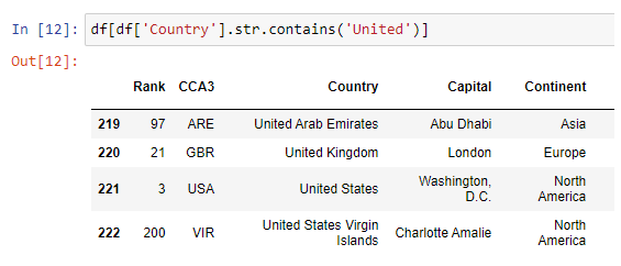
In each result set by now the leftmost column was automatically generated integer index. However, we can specify a custom index by defining an index column, using set_index() function:

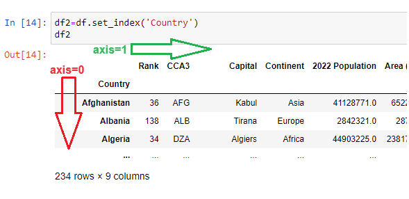
Index column can be understood as "row name" column, or a label for each row - such as header is in fact a "column name" row, or a label for each column. In Excel we usually have headers in our data set, and rows are automatically numbered by Excel with row names, which is the same in DataFrame object. So if convenient, we can set the leftmost column as "row name" column and that would actually be a DataFrame index.

Filtering items by axis 0 (rows) or by axis 1 (columns) is done using filter() function, specifying the items as an argument containing a list. Axis is automatically chosen if we don't specify it (in this case axis=1).

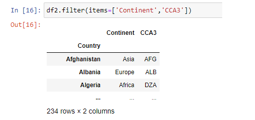
To be on the safe side it is always better option to specifiy an axis. For instance, we can search rows for value of specific country within the indexing column:

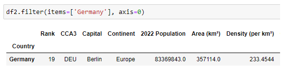
It can be passed a string as a value for like argument in filter() function:

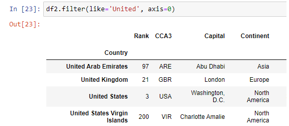
Filtering with specific value in index column can be done using loc[] function:

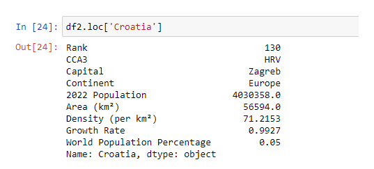
Unlike loc function, the iloc[] function - that is integer loc - locates specific row based on its index:

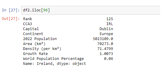
Data sorting (ordering)

Sorting data in pandas can be done by single or multiple columns, in ascending or descending order, that can be specified for each column in particular. As a basic datase for demonstrating data sort will be used subset with Rank lower than 10:

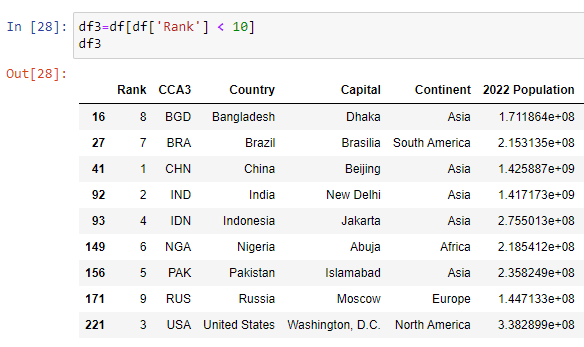
Sorting data by single column can be done the following way (ascending order is by default), using sort_values() function:

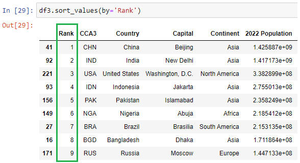
Sorting data by multiple columns, let'say by Country ascending and by Continent descending is done as shown in the image below:

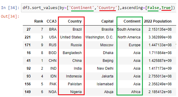
Data indexing

Data indexing in pandas means selecting particular subsets of data (such as rows, columns, individual cells) from that dataframe. The row labels, called dataframe index, can be integer numbers or string values. Since both the dataframe index and column names contain only unique values, we can use these labels to refer to particular rows, columns, or data points of the dataframe. Indexing can also be known as Subset Selection.

The code used in this section is available on GitHub repository.
Dataset will be loaded from CSV file. By default, there is an integer column containing automatically generated 0-based index. This can be changed by very data loading through passing an index_col argument. Data loaded in DataFrame are now indexed as defined, and that can be reset to default by using reset_index() function. To do this on the original DataFrame, not on a copy, inplace argument is to be passed with a value of True. Another way to define an index is set_index() function:

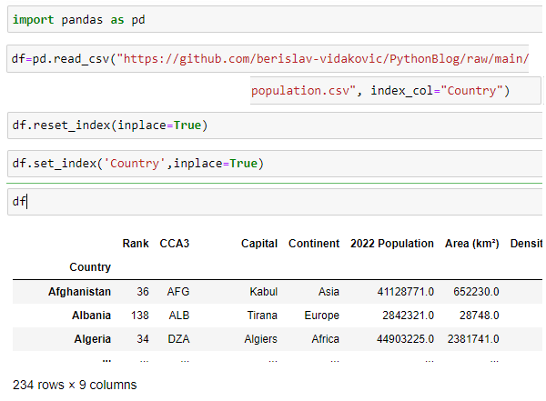
Searching through an index is done by using loc[] and iloc[] functions, as described in the previous article. There can be created multiple index i.e. index containing multiple columns.

To list all columns in the dataFrame object it can be used columns attribute :

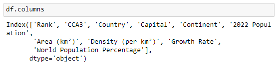
In the following example it will be taken subset of countries with the rank lower than 10. On this subset there will be created multiple index, on Country and Continent column.

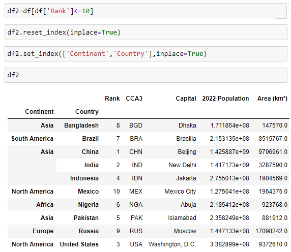
After calling sort_index() function Continent index will be grouped sorted descending and Country index sort ascending within it:

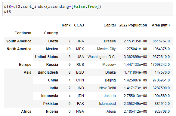
Data connection modes in Power BI

Sunday, 20.08.2023

There are many so called 'school examples' out there that are trying to be used to teach us about Power BI features, which is a standard way of documenting a software tool and presenting its features. School examples are usually easy data sets with a few records and a few fields, nice & easy to understand requiring not much effort. But in the real world projects business logic or business rules are the hardest part and the most important to comprehend. Working with Power BI becomes easier the closer you are to the data that you’re working with and the more relevant that data is to you and to your organization. Power BI is visual reporting software aimed at non-technical users. There are several ways to share Power BI report with users:

by sending them in .pbix file directly (per e-mail/some other way) or publishing this file to the web

by letting users subscribe to the report via Outlook so they receive e-mails

by adding the report as a tab within MS Teams, or outputting as a PowerPoint

This comes at the end of PBI report creation, but at the beginning it is a critical decision to select a way to connect to data source.

Connecting Power BI to Data Source

it is possible to enable a data source to visualize data by PBI report in many different ways, there are few options:

Connect to an existing data set

Import from XML or CSV file

Create a new data source from scratch

Load an application

Upload a power BI PBIX file

Connect to an existing data set and import i.e. the first and the second options are the ones presented here. There are following data connection modes in Power BI

Import -loaded data are imported in PBI cache. Visualizations and reports are created using that cached data. When data source (Excel workbook) gets updated, the way reports gets updated is that the cache itself has to be refreshed with new data from the data source

Live connection -data source is quering directly, but it lives in Power BI service => much faster option than a direct query. Usual data sources are SQL Server Analysis services, Dataverse, Common Data Service (legacy) or PBI datasets published to powerbi.com

Direct query -data are not imported into PBI cache. Visualizations / reports are created using the data source, PBI goes back to the data source we are connected to and relies on it for the data – no matter when data has changed. When data does change, REFRESH is needed. Each time you open or create a report, the data source is queried, you’re going back to the data source =>SLOWER than import option. This option is used when dealing with data too big for import and needed up-to the-minute data.

Feature notes in Power BI

There are two data visualization types - reports and dashboards - that are being created in Power BI, and select which visualisation type to use depends on specific project requirements. There are some common feature as well as some tool-specific ones, as shown in comparison feature list below.

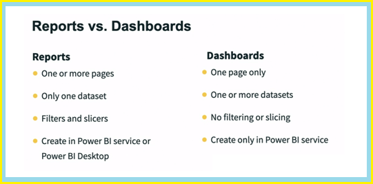
Regarding features on a tool level, there are Power BI Desktop and Power BI Service, that have many common features and specific ones as well, as shown in the image below.

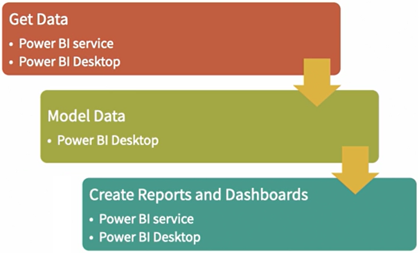
Data modelling or data ETL - extraction, transform & loading - is to be done in Power BI Desktop, in PowerQuery tool, common for Power BI and Excel

Data Warehouse & Data Analysis

Sunday, 23.07.2023

Much of data science & data analysis nowadays is still about gathering the data. Data analyst will spend many working hours in ETL meetings in order for them to be able to ask any interesting questions. It is crucial to understand the terms and challenges to get the data that you need as a data analyst.

Althought relational databases still dominate many organizations used as a backbone for online transactions, there are some limitations, especially when dealing with big data in enterprise analytics where data warehouse is to be considered as central component, since newer applications have challenges that exceed the relational model.

There are following limitations of relational databases:

Lack of flexibility - data analyst often needs a more flexible way to store their data

Schema is required - as relational database relies on a schema, data analyst needs to know a lot about their data before they put it into a database

Require planning - you need to plan ahead, have to know your data format (if your data is for instance text file, audio file or video), organize the fields into tables, and finally tables need relationships

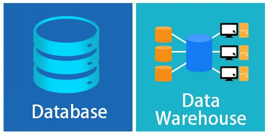
With a Data Warehouse, an enterprise can manage huge data sets, without administering multiple databases. Data warehousing is a method of organizing and compiling data into one database. A data warehouse is a database that is connected with raw-data sources via data integration tools on one end and analytical interfaces on the other. Data integration is the process of taking data from multiple, disparate internal and/or external sources and putting it in a single location - a data warehouse - to achieve a unified view of collected data. Data warehouses collaborate data from several sources and ensure data accuracy, quality, and consistency. Data warehouses store historical data and handle requests faster, helping in online analytical processing (OLAP), whereas a traditional database is used to store current transactions in a business process that is called online transaction processing (OLTP).

Let's consider an example. There is a website of a Music Shop EU that sells musical equipment to musicians in Europe. Site has been very successful and it was bought by a company Music Shop Global that sells musical equipment worldwide. That company has one warehouse for all their websites. They want to take the data from your website and combine it with all their other websites. The company will do something called ETL which stands for extract, transform and load. They'll pull the data from all their websites then they'll load the data into their Enterprise Data Warehouse. The company will extract the data from your website in a standard format then they'll transform the data into something that works well with their data warehouse. Their warehouse could have a different schema than yours. Their data analyst will spend most their time scrubbing and joining the data so it will fit. Finally, they'll load the transformed data into the data warehouse.

While the typical database is focused on working with data in real-time, a data warehouse is focused on analyzing what already happened. Data warehouse is optimized for analytical processing. It's an OLAP database focused on creating reports. Data warehouses are specifically intended to analyze data. Analytical processing within a data warehouse is performed on data that has been readied for analysis - gathered, contextualized, and transformed - with the purpose of generating analysis-based insights.

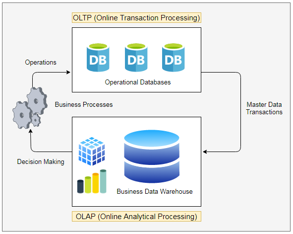
A computer scientist William Inmon, who is considered the father of the data warehouse, first defined Data Warehouse in his book "Building the Data Warehouse" (1992, with later editions). He created the accepted definition of a data warehouse as collection of data in support of management's decisions. According to his definition, these are 4 features of data warehouse

Subject-oriented - They can analyze data about a particular subject or functional area (such as sales). It provides you with important data about a specific subject like suppliers, products, promotion, customers, etc. Data warehousing usually handles the analysis and modeling of data that assist any organization to make data-driven decisions.

Integrated. Data warehouses create consistency among different data types from disparate sources. Different heterogeneous sources are put together to build a data warehouse, such as level documents or social databases.

Nonvolatile. Once data is in a data warehouse, it’s stable and doesn’t change. This means the earlier data is not deleted when new data is added to the data warehouse. The operational database and data warehouse are kept separate and thus continuous changes in the operational database are not shown in the data warehouse.

Time-variant. Data warehouse analysis looks at change over time. The data collected in a data warehouse is identified with a specific period.

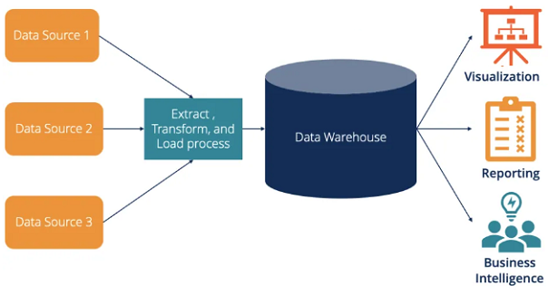
Data warehouses offer the unique benefit of allowing organizations to analyze large amounts of variant data and extract significant value from it, as well as to keep a historical record. It centralizes and consolidates large amounts of data from multiple sources.

There are following main advatages of data warehousing:

Cost-efficient and provides quality of data

Performance and productivity are improved

Accurate data access and consistency

Its analytical capabilities allow organizations to derive valuable business insights from their data to improve decision-making. Over time, it builds a historical record that can be invaluable to data scientists and business analysts. Because of these capabilities, a data warehouse can be considered an organization’s “single source of truth.”

Database normalization - 1NF, 2NF and 3NF

Sunday, 18.06.2023

Although the world of technology has been evolving at a rapid pace, there are still some rather old foundation mathematical concepts in the heart of technology that enable this all to work well. One of them is database normalization that is defined 50 years ago by Edgar F. Codd and contains 3 rules for organizing data in a database. Normalization process should be revisited whenever there's a change to the schema or the structure of the DB.

Database Normalization is a standardized method of structuring relational data that leads to a more efficient database, by helping to avoid complexities and maintain DB integrity. Also known as vertical partitioning or column partitioning, it involves splitting a table into multiple smaller tables based on a subset of columns. The main purpose of database normalization is to improve integrity, minimize redundancy by eliminate duplicates and organize data in a consistent way. It is important to arrange entries in DB in order for other maintainers and administrators to be able to read them and work on them. There are 3 normal forms - 1NF, 2NF and 3NF - that are cumulative, meaning each one builds on top of those beneath it.

Normalization entails organizing a database into several tables. The process of displacing and reorganizing fields in a table is called vertical partitioning and it is performed by creating a new table, pulling fields out from the original table to the new table, and connecting new and original tables with a one-to-many relationship.

1NF - the first normal form

For DB table to be in 1NF it must meet the following requirements:

Atomicity - a single cell must hold only one value, not more

There must be a primary key for unique record identification

No duplicated records or fields

Consistent data type must be enforced for each field

There is an example which shows better the normalization process.

2NF - the second normal form

The second normal form has the following rules:

Primary key of the table is a single field (no composite key)

Each non-key field must depend on the value of the key

After 1NF there still can be data redundancy that has to be eliminated by refactoring DB to the 2NF. This means that each field must be describing only the entity the table contains, and all other fields have to be pulled out to another table created for them.

3NF - the third normal form

The 3NF has only one rule:

Each non-key field must depend ONLY on the value of the key

After reducing model to 2NF all fields depend on the key value, however it is still possible that some fields depend not only on the key value but also on each other. This transitive partial dependency is to be adressed with 3NF. In the table that meets 3NF requirements no values can be stored if they can be calculated from another non-key field. Each non-key field in a record should represent something unique about a record.

Example of DB normalization to 3NF

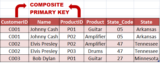
The table above is in 1NF. All entries are atomic and there is a composite primary key. As fields "Name", "State_code" and "State" are dependent on part of primary composite key ("CustomerID") and the field "Product" depends on part of primary composite key too ("ProductID") the table is not in 2NF. To make it 2NF the table should be separated to more tables, in which primary key will be single-field and non-key fields will be dependent on primary key

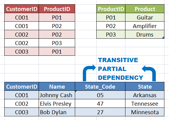
The model above is now in 2NF. There is however one more transitive partial dependency - Field "State" is not only dependent on primary key but also on "State_code" field. After separation in the new table the model will be in 3NF

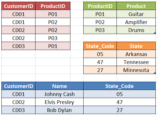
The model above is in 3NF as it is in both 1NF and 2NF and all non-key fields depend only on the primary key.

Excel functions, tips & tricks

Sunday, 21.05.2023

Microsoft Excel, an essential tool in data analytics, is a spreadsheet program and one of the first things aspiring data analysts has to master. There are some most relevant Excel functions used in data analysis, as well as some general-purpose useful functions described in further text. To use Excel properly, a good understanding of the following program’s formulas is neccessarily required.

CONCATENATE or & operator - These functions are to be used to join 2 or more strings. Both CONCATENATE and "&"" operator work the same way, taking as arguments partial strings that can be passed directly or as cell reference, and returning as a result joined passed strings together

LEFT, RIGHT, MID functions - String functions for extracting left, middle or right portion of the passed string. For LEFT and RIGHT functions argument is number of character from the left or from the right, and for MID function arguments are starting position and number of characters from the starting position towards the end of the string

SUBSTITUTE, LEN, TRIM functions - Using SUBSTITUTE function it can be replaced specified substring within passed string with a new string. LEN function returns number of characters in passed string and TRIM function removes all blanks from the left and from the right of the string

UPPER, LOWER, PROPER functions - Converting passed string to upper case, lower case or proper case (each word starting with upper case letter and other letters left lower case)

String and formula in cooperation using INDIRECT -Referencing to particular cell can be done indirectly as well, by building cell reference string (such as "B2" or "C4") from variables, either passed directly or as cell contents

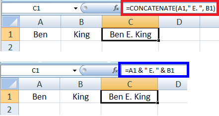
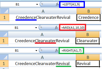
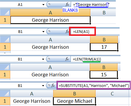
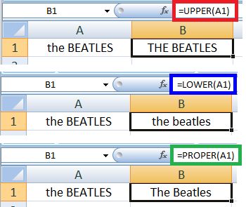
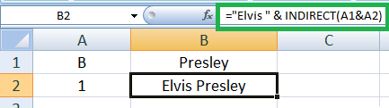
Useful keyboard shortcuts
---------------------------------
-Ctrl+Shift+8 - select region around current cell. Region is rectangular area (range) bounded by any combination of blank rows and blank columns
-Ctrl+T - convert currently selected range into a table
-Ctrl+PageDown - move forward from the current to the next worksheet
-Ctrl+ArrowDown - move to the last non-empty cell (before the first empty cell) in the column
-Ctrl+Shift+ArrowDown - select all cells from the current to the last non-empty cell (before the first empty cell) in the column

COUNT, COUNTA functions - For counting number of cells that contain any value (non-blank cells) it is to be used COUNTA function, and for counting non-blank cells that contain only numbers it is used COUNT function. Argument can be a range (entire columns such as A:B or rows such as 1:3, or limited range such as A1:B5), a row (entire row such as 2:2, or limited cells within a row such as A1:C1), or a column (entire column such as C:C, or limited cells within a column such as B3:B7).

DAYS, NETWORKDAYS and ISOWEEKNUM functions - Number of days between 2 dates is calculated using DAYS function. First date is included and second date is excluded from calculation (number of days between 10.01.2023 and 15.01.2023 is 4). For calculating only working days - excluding weekend days - between 2 dates it is used NETWORKDAYS function, including both first and second passed dates. Acc. to ISO standard week number 1 of particular year is defined as the first week in the year that contain most of days (4 or more week days) from that year. For the year 2023 week nr. 1 is 02.01-08.01 so the function ISOWEEKNUM ("03/01/2023") would return 1 as a result.

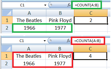
DAYS(date1, date2)
NETWORKDAYS(date1, date2)
ISOWEEKNUM(date1)

IFERROR, IFNA functions - It is good practice to wrap functions within IFERROR or IFNA to define return value for the cases when main function didn't return valid value. By default, Excel would return #N/A value for such cases. Using IFERROR and IFNA is almost the same, with only difference that IFNA catches only #N/A error type and IFERROR cathes all other error types. IFNA is introduced since Excel 2013 so it does not work in previous versions.

Sorting and unsorting data in Excel table - It is common practice to sort data in the table and it's pretty intuitive to find a way how to do it. However, unlike filtering, it is not so easy to revert to original, raw (unsorted) data, if we saved sorted table in the meantime, didn't save backup copy of original data and/or performed many other operations in the meantime. There are 3 recommended ways to enable revert to original data, to be done before sorting (except Undo function, of course): create data backup copy, add helper column and using undo function.

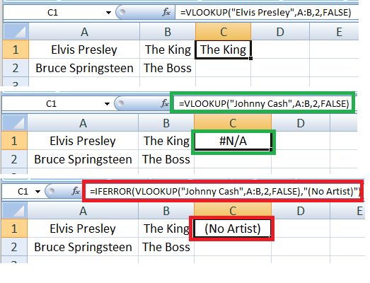
3 ways to enable reverting sorted table to orignial
--------------------------------------------------------------
-Ctrl+Z - UNDO function can be used if sorting was the last operation applied, or among last few applied operations. However, if we need today to revert back to original the table we sorted yesterday, this option would not work
-Backup copy - It is best practice to create backup copy of data before start to modify them. That would prevent any problems with reverting to original
-Helper column - Before very data sorting, there is one column to be added with sequenced values starting from 1 for the first row, 2 for the second row etc. Reverting to original will be done via sorting by this column.

Reading files in pandas (csv, txt, json, xlsx)

Sunday, 09.04.2023

This article will explain reading data from different file formats: CSV format, text format, Excel format, JSON format. Each reading function returns a DataFrame object which is 2D-array such as Excel worksheet. All files used in the article are stored in GitHub repository, as well as the code from all examples , that is stored in jupiter notebook format (.ipynb).

Python features covered in this article
---------------------------------------------
-read_csv(header, names, sep)
-read_table(sep)
-read_json()
-read_excel(sheet_name)
-get_option()
-set_option()
-DataFrame.info()
-DataFrame.shape()
-DataFrame.head()
-DataFrame.tail()
-DataFrame['Column_name']

Comma separated value files - CSV

Opening CSV file in Pandas is to be done using read_csv function:

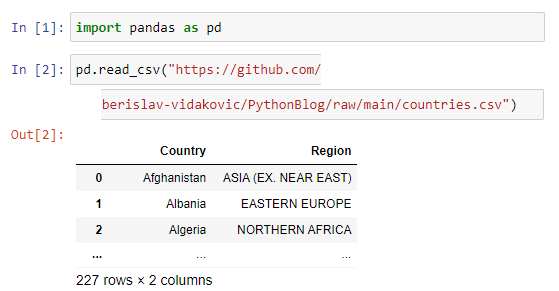
The same result we would get if we used read_table function with a specified delimiter which is comma(,) in our CSV file:

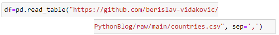
Optionally, if we pass an argument header=None to read_csv function, the first row will not be taken as a header:

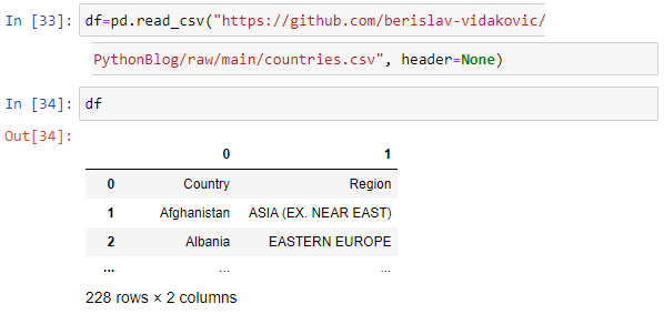
There is also a possibility to set custom header names by passing an argument names=['Land','Bezirk']

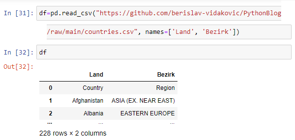
Text files - TXT

To open TXT file it is used read_table function:

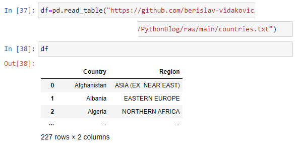
The same result we would get if we used read_csv function with a specified delimiter which is TAB in our TXT file:

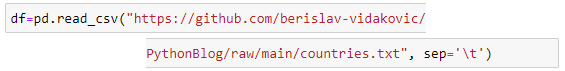
It can be shown only particular column using square brackets operator with specifying column name:

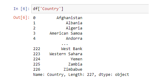
JSON files

To open JSON file it is used read_json function:

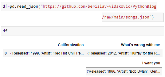
Using Shift+TAB key combination when positioned within function argument area it's opened a box that shows all parameters and their descriptions:

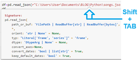
Excel files

Opening an Excel file in Pandas is to be done using read_excel function:

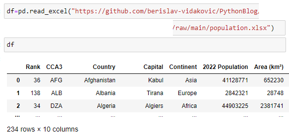
By default, the first worksheet is opened. It is also possible to open a particular sheet, by specifying sheet_name argument:

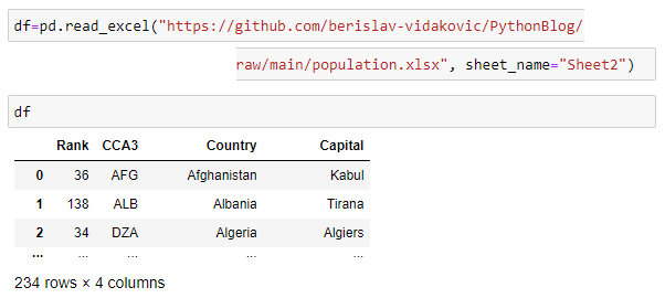
Using info() and shape() functions there are information about our data frame:

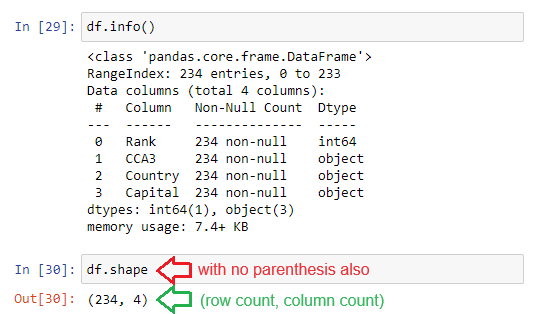
To see only first or last specified number of rows we are using head() or tail() functions:

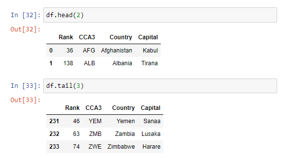
To check how many rows or columns are shown it is used get_option function and to change the number of rows or columns shown it is used set_option function, passing the argument accordingly:

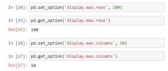
Power BI basics

Sunday, 12.03.2023

Althought both Power BI and Excel are two very popular tools and both have a lot of features that make them great for data analysis, there are many advantages of Power BI compared to Excel, worldwide well known and higly used spreadsheet tool. Power BI is more efficient in handling the capacity of data quantity since it has faster processing than Excel. Power BI is more user friendly and easy to use than Excel. When dashboard building completes in Power BI, report can be published to the end-users with cloud-based services, unlike sharing the large data in Excel via email or any online sharing tool. Reports in Power are more visually appealing, customized, and interactive than in Excel

Like in Excel (since version 2010) there are in Power BI as well the 2 ways of filtering data in Matrix tables (known as Pivot tables in Excel): hard filters - created by adding a filtering field to filter section, and soft filters - Slicers. Slicers are more flexible an more transparent than hard filtering. When there is more than one value in the field selected for filtering it can be seen in the slicer.

To select more than one item in the slicer, after selecting the first item press and hold Ctrl button and then select another items

Slicers enable connection to more than one matrix tables allowing the user to apply filter on multiple Matrix Tables with one click of a button. They work great for touch screen devices allowing a great user experience on mobile as well.

There is an example that will show some basic Power Bi features. Data source is Excel table containing albums released by Bob Dylan in the first 5 years of his career. Table contains 4 fields and 71 records, there are few top records and few last records shown in the image below. Entire table can be downloaded from this link.

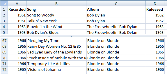
Creating matrix table in tabular view

For data model shown in this example, there will be 2 data fields added to matrix table: Album name and Released year. Since both fields will be added to Rows section, by default matrix table will look as shown in the image below:

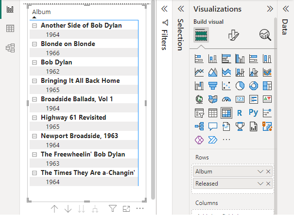
To set a matrix table to tabular view as known in Excel, there are following steps as shown in the image below:

Select Matrix Table (1)

In Visualizations section select Format visual button (2)

Select Row headers option (3)

Select Options section (4)

Set Stepped layout option to OFF (5)

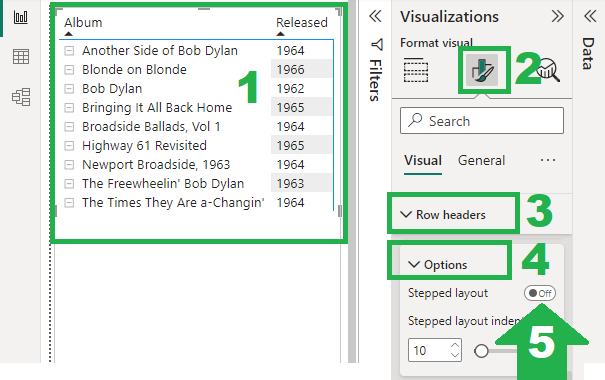
Adding slicer in list style

When inserting a slicer in Power BI and adding data field wanted to be filtered by (field Released), the default slicer view looks as shown in the image below

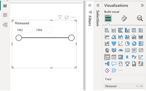
To set a slicer style to list view as known in Excel, there are following steps as shown in the image below:

Select Slicer (1)

In Visualizations section select Format visual button (2)

Select Slicer settings option (3)

Select Options section (4)

Select Vertical list option in dropdown list (5)

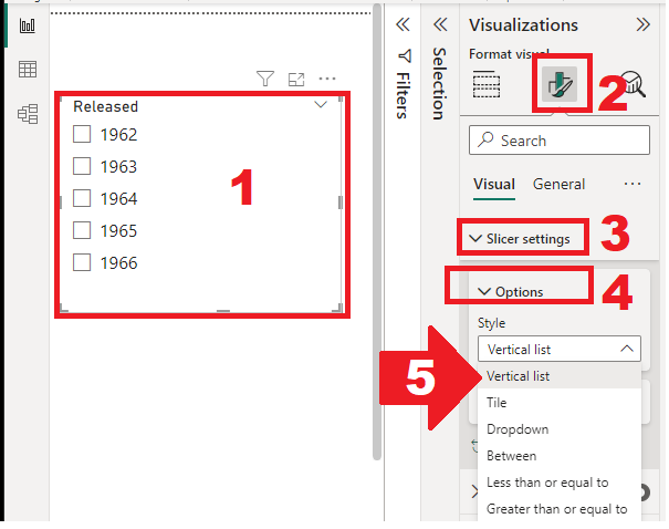
Connecting/disconnect slicer to visual

Like is Excel as well, in Power BI it is also possible to define connections between slicer and other visuals. In order to select visual to be or not to be connected to the particular slicer there are following steps:

Select Slicer (1)

Select Format option from menu (2)

Select Edit interactions option on the left (3)

Select Right button for visual NOT to be connected with slicer (4)

Select Left button for visual TO BE connected with slicer (5)

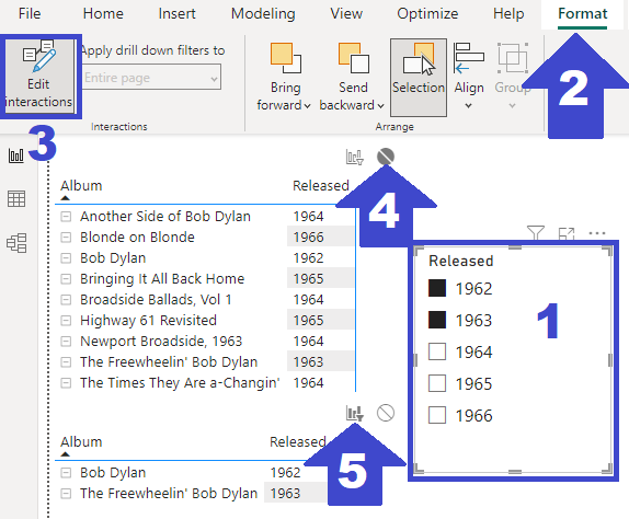
The upper matrix table thet is not connected to slicer shows all Bob Dylan's albums released in the first 5 years, and the lower matrix table connected to slicer shows only filtered data shown on slicer i.e. albums released 1962 and 1963.

Using SQL for creating Pivot table

Sunday, 19.02.2023

There is one regular task in Data Analysis that every data analyst will usually be assigned to from their management. It is required to create a report that shows YTD delivered items grouped by delivery destination. Let's say there is a table containing all delivered items, and in that table there are both needed fields - Quantity and Destination. Table is in Excel, so the task looks simple & easy - create Pivot table with Destination field in rows and sum of delivered items in Values....yes, but! There would be no problem or neccessity to write this article and to think about using "complicated" SQL instead of "simple" Pivot table tool - if there is an example like the following:

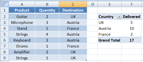
If the real world cases were like this one school example, we would not need a computer at all, all would be get done by hand in a minute! But the real world examples are usually a little bit bigger. One table as a flat file can be generated weekly from the system.

To reach the last row in the table i.e. to check how many records are there in a big Excel table, the easiest way is to use key combination
Ctrl + Arrow-Down

There are nearly 400,000 records in the weekly table...and that's the point where an Excel nightmare starts.

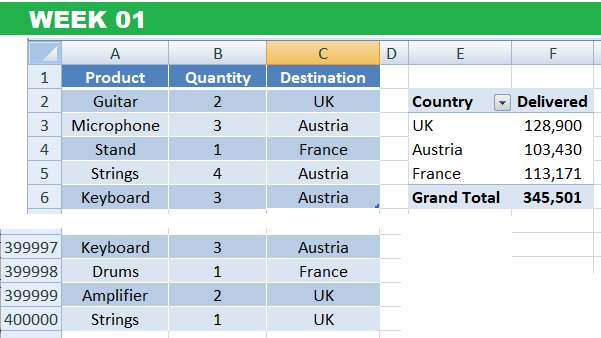
Not to mention how long it takes to open one file that contains data for one week, but with the row limit of slightly above 1 milion it could be placed at most 2 weeks of delivery in one Excel file.

Total number of rows on a worksheet in Excel file is 1,048,576 rows

Who would like to imagine how long then would it take to open a file with almost 1 milion records? I would rather not. And if the task was set for the last year in December and not in February, there would be 50 week tables, not (only) 8. Anyway, let's imagine in December I get the task to refresh this report...There is no way to get whole-year delivered items in one Excel table. Opening one by one just to create a pivot table would last ...well, pretty long. It would be neccessary to open 50 times a table for each week, to create weekly pivot table, and then join them to get a yearly picture.

This is the point that SQL jumps in. All Excel table are to be imported to RDBMS - for instance, as linked tables to MS Access database.

CREATE VIEW View_Year2023 AS
SELECT * FROM Week01
UNION ALL
SELECT * FROM Week02
UNION ALL
...
SELECT * FROM Week50

With one SQL statement contains more SELECT statements connected with UNION keyword it is created a view (saved query) that was a reference to one table with all delivered items. Yes, there are cca 20 milion records...not so much for SQL, but way too much for Excel.

SELECT Destination AS Country,
SUM(Quantity) AS Delivered
FROM View_Year2023
GROUP BY Destination

Created view is selected as a data source for SQL statement that creates a Pivot table...And voila!

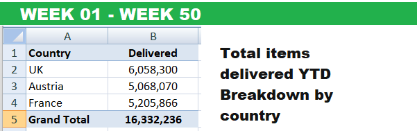
OK, Access is not the fastest RDBMS in the world, but it saved much of time and energy.

Python libraries - pandas

Sunday, 15.01.2023

Pandas is a Python library used for working with data sets. It has functions for analyzing, cleaning, exploring, and manipulating data. The name "Pandas" has a reference to both "Panel Data", and "Python Data Analysis" and was created by Wes McKinney in 2008.
There is an example from the music world that will be used to demonstrate substantial feature of pandas library as tool for Data Analysis. The data source is a table containing top 12 Bob Dylan songs, saved in a CSV file, shown in the table below:

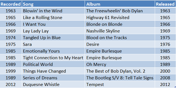
The first step is to open the CSV file that is our data source. Return value of the function reading CSV file is Data Frame object.

import pandas as pd
dfBob = pd.read_csv("https://barrytheanalyst.eu/
Portfolio/DataSource/BobDylanTop12.csv")

To check if the first row is recognized as a header, we can try to access particular column by header name using Series function

pd.Series(dfBob['Song'])

The result of printing return value of Series function will be as shown below, which means first row is recognized as headers

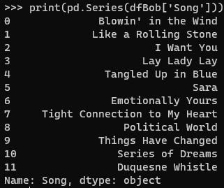
If there would have been bigger table, Python would have shown only part of the table, only number of first row that is defined by specific parameter pd.options.display.max_rows

The first 5 rows by default is printed using head() function and the last 5 rows using tail() function. It can be passed parameter to these functions as well, to specify exactly how many rows to display. Detailed information about table - number of rows, columns etc. - in data model will be shown using info() function

dfBob.head()
dfBob.tail()
dfBob.info()

Series can be converted to list using tolist() function

lsSongs=pd.Series(dfBob['Song']).tolist()

Accessing rows and columns in DataFrame

Accessing ROWS in the table by index is done using iloc() function of dataframe object, passing 0-based index of the particular row. It can be passed more than one index to reach selected rows identified by indexes.

dfBob.iloc[3]
dfBob.iloc[[4,5]] #doube square brackets

When requested 1 row result will be displayed in 'design view' and when requested more than 1 row, results will be displayed in 'table view', as shown below

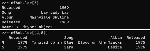
Accessing COLUMNS in the table by index is done using iloc() function of dataframe object, passing 0-based index of the particular column after : and comma.

dfBob.iloc[:,1] #column with index 1=Song

There will be following result as output of column accessing

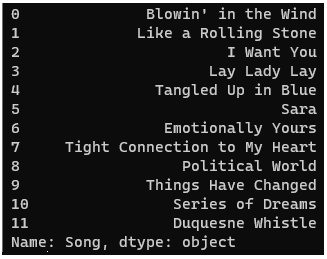
Data cleaning & basic statistical functions

Empty cells can potentially give you a wrong result when you analyze data. One way to deal with empty cells is to remove rows that contain empty cells, and since data sets can be very big removing a few rows will not have a big impact on the result. Removing records contain NULL values can be done directly to original data frame, or by creating a new data frame as a copy that will contain no NULL value.

new_dfBob = dfBob.dropna() #copy created
dfBob.dropna(inplace=True) #original changed

Also, it can be specified only particular field to test on NULL values (if no field specified, all records contating NULL values will be deleted)

dfBob.dropna(subset=['Released'],inplace=True)

For each column specified by index (header name) it can be calculated average, median and mean value by calling built-in functions

dfBob['Released'].mean() #avg value
dfBob['Released'].median() #middle value
dfBob['Released'].mode() #most frequent value

Selecting distinct records from DataFrame object

It is not possible to use unique() function when there are 2 fields, and unique() function is used when there is single field handling.

Method pandas.DataFrame().unique() is used when unique values are to be selected from a single column of a DataFrame. It returns all unique elements of a column. It can also be used when there is more than 1 column, in combination with append() function. Since append function will be removed from future versions of Python, it is recommended to use concat() function for this purpose

uniqueVals = (dfMS['Product'].append(dfMS['State'])).unique()

Two columns are merged and distinct records are returned as new DataFrame object.

Aggregate functions in DataFrame

When applying groupby() and some aggregate function - sum(), mean(), min(), max(), count() - it is possible to be returned Series object or DataFrame object as well.

Return value is Pandas Series if used single brackets
data.groupby('Recorded')['Song'].count()

Return value is Pandas DataFrame when used double brackets
data.groupby('Recorded')[['Song']].count()

Sorting records in DataFrame

Sorting records in DataFrame object is done by using sort_values() function. This function by default creates a copy of DataFrame object, not changing original (unsorted) DataFrame object. Original object can be changed by passing an argument inplace=True, or sorted DataFrame can be saved back to original, or some other DataFrame object.

dfBob.sort_values(by='Song',inplace=True) #org changed
dfBS = dfBob.sort_values(by='Song') #copy created

Data Analisys roles & goals

Sunday, 18.12.2022

There are quantitative (numeric) data and qualitative (descriptive) data that can be processed with 3 types of data analysis: descriptive, predictive and prescriptive one. Descriptive data analysis deals with events that has happened, predictive data analysis deals with that what might happen and prescriptive data analysis tells stakehoders what they should do in the future. Essential tools and programming languages used for data analysis are Excel, SQL, Python and Power BI.

The are 3 types of data:

Structured data - data with formally defined scheme, such as database with tables containing fields. Structured data fits neatly into tables or spreadsheets.

Semistructured data - structured, but flexible about field defining, such as e-mail, blog, XML or JSON

Unstructured data - schemeless data, such as photo, video, audio or PDF

Data roles, Analysis & more

Data analyst works with structured data while data scientist works with unstructured data. In short: Data analysts turn raw data into meaningful insights. Main skills that data analyst has cover DB tools, programming languages, data visualization, statistics and math. Job functions of data analysis role are analizing data for insights and communication of those insights to stakeholders.

Tools-agnostic skills that every data analyst has are the following:

understanding the basic questions

finding & gathering data to answer the questions

understanding the quality of data

determine what data is important

create valid data through calculations

presenting information clearly

To make life of data analyst easier there is data engineer that has the following tasks:

builds datasets

translates large amount of data into datasets - into formats that can be processed & analyzed

knows how to refine datasets into smaller sets

has more access to data and understands security and privacy

gathers data from different sources

optimizes DB for analysis

removes corrupt files and repairs the pipeline

automates tasks and pipelines that store data in suitable format

has a solid knowledge of programming languages & technologies

Data architect is data engineer with more system, more server and more security strategy knowledges.

senior visionaries who translate business requirements into technology requirement and

define data standards

The most universale data role is Data worker who has the following tasks:

consumes & works with data regularly

performs data manipulation

presents data as a form of their everyday work

prepares report for manager - the only difference is new data

exports data from data system to CSV and Excel - there procedure of data worker starts

Compared to data worker, data analyst:

has more access to data

models the data

automates the flow of data

analyzes and presents data on a deeper level

Common tasks of data analyst and data worker are:

gathering data

manipulate data to meet requirements

reporting the outcome

Essential definitions in Data Analysis

ETL process - Extract, transform, and load - plays a critical role in Data Analysis. It is the process of combining data from multiple sources into a central data repository, using a set of business rules to clean and organize raw data and prepare it for data analytics, containing the following steps:

EXTRACT data from its original source

TRANSFORM data by cleaning it, removing duplicates etc.

LOAD data into a target database

There is a difference between data literacy and data fluency. Data literacy is the ability to read, speak, listen and understand data. Data fluency is the ability to create something - tools, reports, visuals and data sets - beyond just being able to understand, read and use it. Data governance covers access to information, source of truth and masters data management

Data quality is measured with the following

completeness (are there all, missing, usable)

consistency (in other systems too)

validity (meet the requirements, format OK)

accuracy

Data that meets quality requirements can be used to make important, data-driven decisions

There is business intelligence (BI) that deals with collecting and housing data about current operations - speed per mile, average miles per hour. It helps to understand where we stand on any given day, and to answer the question 'how are you perorming today?' Tool are used to build BI, but they don't provide it by themselves. BI ensures that companies stay focused on their primary target to successfully get where they want to go. Business analysis (BA) is about analyzing data and creating more of it (track running info, for instance). It analyzes trends in order to predict future outcomes. It is a more statistical-based field, where data experts use quantitative tools to make predictions and develop future strategies for growth. Data analysis (DA) analyzes and captures data to compare over time. Based on its historical data and BA insights it is searched for an answer 'how you potentially perform in the future?'

Key performance indicators (KPI) is a common tool to display the metrics used for the overall health of the organization and the targets for BI. There is a potential trap as a possible result of overthinking known as analysis paralysis that is bo be overcome by building approach, thinking through standard questions, using critical thinking and practicing active listening.

Data is defined with 3 components: value, type and field. Integrity of data is accomplished after removing duplicates. Data profiling is used on every data set before beginning to analyze the data when we want to know how much data we have in set. It helps validate our numbers and shows what we're facing when we're ready to transform our data. High-level profiling enables insight of the characteristics of the working data that that is prerequisite for data transformation.

Common mistakes for new data analyst

Take not enough time to understand the data

Not looking for duplicates

Not doing preliminary math (SUM, AVG, COUNT)

Not capturing record count

Not document questions and follow-up answers

Not verifying numbers with some other method

Not asking questions out of fear

Not asking for documentation

Best practices for Data Analyst

Don't make up an answer (no guesswork)

Don't publish until you verify results

Be prepared for meeting, use time effectively

Take notes of everything

Provide detailed info about what you're presenting

Don't put data on-screen before diving in

Use slide deck in presentation to keep pace

Reiterate key points

Ask others for their best practices

Branching, loops & functions

Sunday, 20.11.2022

This article will explain functions, loops and branching in Python. Function is a block of statements that runs the specific task. The idea is to put some commonly or repeatedly done tasks together in a function so that instead of writing the same code for different inputs, we can call the function to reuse code contained in it. Loop is used to execute a block of statements repeatedly until a given condition is satisfied. Branching is using conditions to determine which set of instructions to execute. The code from all examples is stored on GitHub Repository in Jupiter Notebook format (.ipynb).

Python features covered in this article
---------------------------------------------
-def
-if/elif/else
-type()
-for/else
-while/else/break/continue
-map()
-list() for conversion to list
-lambda function
-get() function on dictionary
-tuple() for conversion to tuple

Functions

Functions in Python are defined with a keyword def. Function can have no parameters or many parameters. When calling a function, arguments can be passed with or without keywords and, when passed with keywords, that has a priority toward the order defined in parameter list in function declaration/definition. There are few examples:

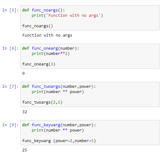
There is a flexibility in Python regarding number of function arguments - it is possible to have arbitrary number of arguments. The passed arguments are referenced in the function definion using 0-based index. Arguments can be passed either directly or by using a tuple defined previously. If used a keyword arbitrary argument option, then passed arguments are referenced using string specified when function called:

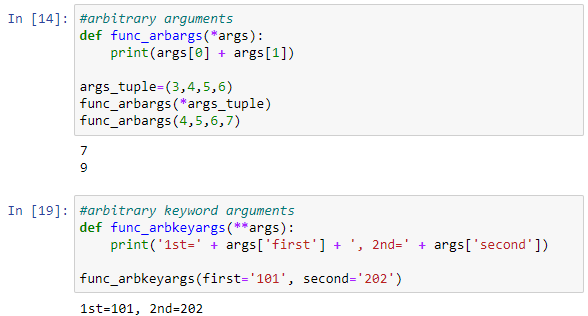
Branching & Loops

Branching using if-elif-else is pretty intuitive:

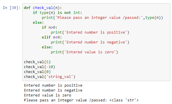
Loops for and while are used for iterating in an array. There are examples of for loop iterating in an integer array and in dictionary:

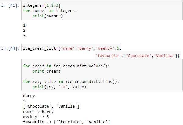
Loop while is running while the condition defining in the loop beginning is True. Both for and while loops can have elese statement at the end, that runs when loop is finished to the last iteration.

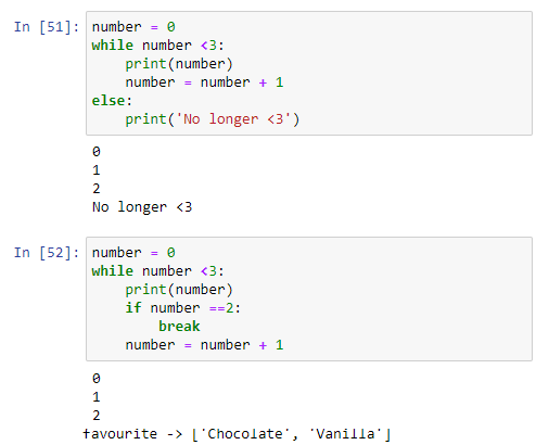
Else statement doesn't run if there is a break in the loop. If there is a continue statement, it will skip the current iteration but while loop will still be running to the end, including else statement:

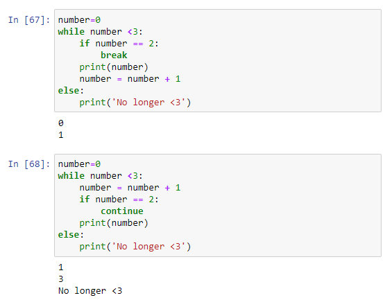
Function map()

Function map() allows us to map a function to a python iterable such as a list or tuple. Function passed can be built-in or user-defined, and since it is not a function calling, just passing an adress, it's to be used a function name with no parenthesis(). Lambda function is an anonymous function defined in one line of code, and it is especially suitable for using in map() function. The code from all examples in this section is stored on GitHub Repository in Jupiter Notebook format (.ipynb).

Map function helps us to be more explicit and intentional in code. Map function takes as arguments a function and an iterable on which elements passed function will be performed. It returns map object which can be converted to list using list() function or to tuple using tuple() function, as well as to many other types or classes. There are 3 examples that shows using map() function compared to other possible solutions in creating a new list that contains length of elements in the list:

Using lambda function in map

Using lambda function is a practical way for defining a map function, because it requires less lines of code and reduces dependency (user-defined function has to be defined previously if using a standard way). There are 2 examples illustratiing both ways, function passed to map() calculates cube of each list element:

Applying map() to many lists, a dictionary and tuple

We can pass more iterables to map() functions, for instance two lists and define with a lambda function an operation to be performed on elements of each one. List can contatin dictionary elements, which can be safely accessed using get() function and passing 0 for the case that an element doesn't exist. Lambda function passed to map() function can return tuple as well. There are examples:

SQL essential features

Sunday, 23.10.2022

Structured query language (SQL) is a programming language for storing and processing information in a relational database. It was initially developed at IBM by Donald D. Chamberlin and Raymod F. Boyce in the early 1970s, after learning about Codd's relational model. SQL is used to create a database, define its structure, implement it, and perform various functions on the database. SQL is also used for accessing, maintaining, and manipulating already created databases.

SQL statements are divided into 3 categories: data control language (DCL), data definition language (DDL) and data manipulation language (DML). DCL deals with controls, rights, and permission in the database system, it defines the structure or schema of the database. DDL is used to build and modify the structure of your tables and other objects in the database. DML is used to work with the data in tables, to deal with managing and manipulating data in the database. They are used to query, edit, add and delete row-level data from database tables. There are examples of usage mostly as DML and few of using it as DDL

Use the NOT keyword to select all records where City is NOT "Berlin".

SELECT * FROM Customers WHERE NOT City = 'Berlin';

Select all records from the Customers table, sort the result alphabetically (and reversed) by the column City (or alphabetically, first by the column Country, then, by the column City).

SELECT * FROM Customers ORDER BY City;
SELECT * FROM Customers ORDER BY City DESC;
SELECT * FROM Customers ORDER BY Country, City;

Insert a new record in the Customers table.

INSERT INTO Customers (CustomerName, Country)
VALUES ('Hekkan Burger', 'Norway');

Select all records from the Customers where the PostalCode column is empty (or not empty).

SELECT * FROM Customers WHERE PostalCode IS NULL; SELECT * FROM Customers WHERE PostalCode IS NOT NULL;

Copy all columns (or only some columns) from one table to another table:

INSERT INTO tab2 SELECT * FROM tab1 WHERE condition;
INSERT INTO tab2 (column1, column2, column3, ...)
SELECT column1, column2, column3, ...
FROM tab1 WHERE condition;

Update the City column of all records (or only the ones where the Country column has the value "Norway") in the Customers table.

UPDATE Customers SET City = 'Oslo';
UPDATE Customers SET City = 'Oslo'
WHERE Country = 'Norway';

Update the City value and the Country value.

UPDATE Customers SET City = 'Oslo', Country = 'Norway' WHERE CustomerID = 32;

Delete all the records from the Customers table where the Country value is 'Norway' (or all the record).

DELETE FROM Customers WHERE Country = 'Norway';
DELETE FROM Customers;

Use the MIN function to select the record with the smallest value of the Price column, and other aggregate function for largest, sum and average value.

SELECT MIN(Price) FROM Products;
SELECT MAX(Price) FROM Products;
SELECT AVG(Price) FROM Products;
SELECT SUM(Price) FROM Products;

Select all records where the value of the City column starts / ends with the letter "a" / contains letter “a” / starts with letter "a" and ends with the letter "b".

SELECT * FROM Customers WHERE City LIKE 'a%';
SELECT * FROM Customers WHERE City LIKE '%a';
SELECT * FROM Customers WHERE City LIKE '%a%';
SELECT * FROM Customers WHERE City LIKE 'a%b';

Select all records where the value of the City column does NOT start with the letter "a" / the second letter of the City is an "a")

SELECT * FROM Customers WHERE City NOT LIKE 'a%';
SELECT * FROM Customers WHERE City LIKE '?a%';

Select all records where the first letter of the City is an "a" or a "c" or an "s" / where the first letter of the City starts with anything from an "a" to an "f" / the first letter of the City is NOT an "a" or a "c" or an "f".

SELECT * FROM Customers WHERE City LIKE '[acs]%';
SELECT * FROM Customers WHERE City LIKE '[a-f]%';
SELECT * FROM Customers WHERE City LIKE '[!acf]%';

It can be used underscore "_" operator with "?" for single character interchangebly, and in MS Access only "?".

In MS Access wildcard operator is "*" and not "%" for more characters, but for single character it has to be used "?" only

Use the IN operator to select all the records where Country is/is not either/neither "Norway" or/nor "France"

SELECT * FROM Customers
WHERE Country IN ('Norway', 'France');
SELECT * FROM Customers
WHERE Country NOT IN ('Norway', 'France');

Use the BETWEEN operator to select all the records where the value of the Price column is between 10 and 20 / NOT between 10 and 20 / ProductName is alphabetically between ‘Alpha’ and ‘Delta’

SELECT * FROM Prods WHERE Price BETWEEN 10 AND 20;
SELECT * FROM Prods WHERE Price NOT BETWEEN 10 AND 20;
SELECT * FROM Prods
WHERE ProductName BETWEEN 'Alpha' AND Delta';

When displaying the Customers table, make an ALIAS of the PostalCode column, the column should be called Pno instead.

SELECT CustomerName, Address, PostalCode AS Pno
FROM Customers;

When displaying the Customers table, refer to the table as Consumers instead of Customers.

SELECT * FROM Customers AS Consumers ;

Create the JOIN clause to join the two tables Orders and Customers, using the CustomerID field in both tables as the relationship between the two tables.

SELECT * FROM Orders
LEFT JOIN Customers
ON Orders.CustomerID =Customers.CustomerID ;

Choose the correct JOIN clause to select all records from the two tables where there is a match in both tables.

SELECT * FROM Orders
INNER JOIN Customers
ON Orders.CustomerID=Customers.CustomerID;

Choose the correct JOIN clause to select all the records from the Customers table plus all the matches in the Orders table.

SELECT * FROM Orders
RIGHT JOIN Customers
ON Orders.CustomerID=Customers.CustomerID;

Select all the different values from the Country column in the Customers table.

SELECT DISTINCT Country FROM Customers;

Use the correct function to return the number of records that have the Price value set to 18.

SELECT COUNT (*) FROM Products WHERE Price = 18;

List the number of customers in each country.

SELECT COUNT (CustomerID), Country
FROM Customers GROUP BY Country;

List the number of customers in each country, ordered by the country with the most customers first.

SELECT COUNT (CustomerID), Country
FROM Customers GROUP BY Country
ORDER BY COUNT(CustomerID) DESC;

Write the correct SQL statement to create a new database (or delete a database) called testDB.

CREATE DATABASE testDB;
DROP DATABASE testDB;

Write the correct SQL statement to create a new table called Persons.

CREATE TABLE Persons ( PersonID int,
LastName varchar(255), FirstName varchar(255),
Address varchar(255), City varchar(255) );

Write the correct SQL statement to delete a table called Persons.

DROP TABLE Persons;

Use the TRUNCATE statement to delete all data inside a table.

TRUNCATE TABLE Persons;

Add a column (or delete the column) of type DATE called Birthday.

ALTER TABLE Persons ADD Birthday DATE;
ALTER TABLE Persons DROP COLUMN Birthday;

LOOKUP function family

Sunday, 18.09.2022

There are 3 Excel functions that belong to lookup function family - the older ones are VLOOKUP and HLOOKUP, and the newest one is XLOOKUP. These powerful and easy-to-use functions enables in Excel the functionality which is equivalent to JOIN feature in SQL. The idea is to search a specified value within one array (usually Excel column, although it can be a row too) and to return a corresponding value from another array.

Newer version XLOOKUP has simpler syntax than the older ones since it is possible to define an array directly and independently whether an array is in the column or in the row

XLOOKUP(lookup_val, lookup_arr, return_arr,
[if_not_found], [match_mode], [search_mode])

Required arguments are: lookup_val -value that is searched for, lookup_arr -an array in which search is performed, and return_arr -an array from which value is returned. Optional arguments are: [if_not_found] -return value if searched value not found, [match_mode] -Exact match (0, 1, or -1), and Wildcard match (2) [search_mode] -Search starting at the first or last item (1 or -1), or binary search of sorted lookup_arr ASC or DESC (2 or -2)

While both lookup and return arrays in XLOOKUP function are defined directly as a row or column, in older VLOOKUP and HLOOKUP functions each array is defined indirectly - there is a table (range) that is passed as an argument, its row or column 1 is lookup array and 1-based index of its row or column determines return array.

Older versions VLOOKUP and HLOOKUP have the same syntax with one difference whether search is performed vertically (by column) or horizontally (by row)

VLOOKUP(lookup_val, tbl_arr, col_idx, [rng_lookup])
HLOOKUP(lookup_val, tbl_arr, row_idx, [rng_lookup])

Required arguments are: lookup_val -value that is searched for, tbl_arr -table (range) of information in which data is looked up and from which value is to be returned. Lookup is performed in column or row 1, and return value array is specified in second argument - col_idx or row_idx -index (1-based) of a column or a row in tbl_arr range from which value is returned. Optional argument is: [rng_lookup] -approximate match if TRUE (default value) and values of column or row 1 in tbl_arr have to be sorted ascending, exact match if FALSE and values may be unsorted as well

There are 2 simple examples that illustrate a.m. LOOKUP function family functionality:

In the red table dataset columns are fields and rows are records.

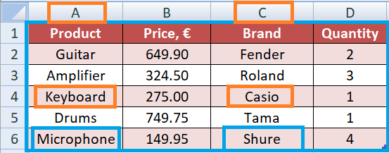
There are examples of XLOOKUP and VLOOKUP functions applied:

=XLOOKUP("Keyboard",A:A,C:C)
=VLOOKUP("Microphone",A1:D6,3,FALSE)

XLOOKUP function returns "Casio" and VLOOKUP function returns "Shure"

In the green table dataset rows are fields and columns are records.

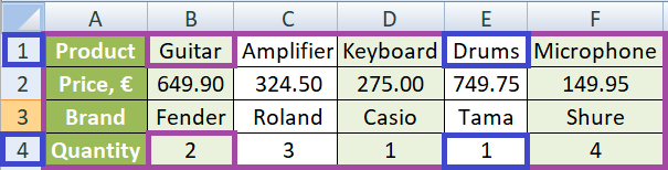
There are examples of XLOOKUP and HLOOKUP functions applied:

=XLOOKUP("Drums", 1:1, 4:4)
=HLOOKUP("Guitar", A1:F4, 4, FALSE)

XLOOKUP function returns 1 and HLOOKUP function returns 2.

There is a brief overview in the table below

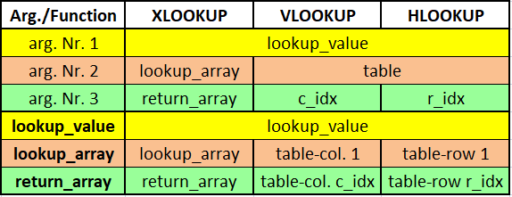
Built-in Data structures in Python

Sunday, 21.08.2022

Data structures allow to organize the data in such a way taht enables storing collections of the data, relate them and perform operations on them accordingly. There are built-in data structures in Python - list, dictionary, tuple and set - as well as user-defined ones such as stack, queue and linked list. There are mutable built-in data structures which means that values of its element can be modified after it is created (list, dictionary and set) and there is immutable data structure as well (tuple) which means element values cannot be modified after a data structure object is created.

List

List is mutable data structure that is ordered so being accessed sequentially by 0-based index. It is created with [square brackets] or by using list() constructor and can contain items of different types. List allows duplicate values

Creating a list

mylist = [] #creates empty list
mylist = [2,6,3] #list of integer values
mylist = list((2,6,3))

Adding and deleting list elements:

mylist.append([11,12]) #[2,6,3,[11,12]]
mylist.extend([15,16]) #[2,6,3,[11,12],15,16]
mylist.insert(1,100) #[2,100,6,3,[11,12],15,16]
del mylist[4] #[2,100,6,3,15,16]
mylist.remove(15) #[2,100,6,3,16]
a=mylist.pop(2) #[2,100,3,16] -returns a=6
mylist.clear() #[]

Accessing list elements:

mylist =[1,3,2,5,4]
for element in mylist:
print(element) #1 | 3 | 2 | 5 | 4
print(mylist) #[1,3,2,5,4]
print(mylist[1]) #3
print(mylist[1:3]) #[3,2] -indexes 1,2 (excl. 3)
print(mylist[::-1]) #[4,5,2,3,1] -reverse order

Accessing by index, getting length and sorting list:

len(mylist) #5 - count of list elements
mylist.index(5) #3 - element with index 5
mylist.count(4) #1 - occurances count of element 4
mylist_s = sorted(mylist) #sort -no change orig.ls.
mylist.sort(reverse=True) #[5,4,3,2,1]

Dictionary

Dictionary is mutable data structure that contains key-value pairs. It is being declared using {curly braces} or by using dict() constructor. Dictionary structure does not allow duplicate members.

As of Python version 3.7, dictionaries are ordered. In Python 3.6 and earlier, dictionaries are unordered.

Creating a dictionary

myDict = {} # empty dictionary
myDict = {'1st':'Python', '2nd':'SQL', '3rd':'DAX'}
myDict = dict(1st = 'Python', 2nd ='SQL', 3rd ='DAX')

Changing, adding, deleting key-value pairs

myDict['3rd'] = 'PowerBI-DAX' #modify
myDict['4th'] = 'C++' #add new
a=myDict.pop('3rd') #delete item with specified key
b=myDict.popitem() #delete last key-value pair
myDict.clear() #empty dictionary

Tuple

Tuple is immutable data structure that is created with (parenthesis) or by usng tuple() constructor.

Creating a tuple

myTuple = (1,2,3)
myTuple = tuple((1,2,3))

To create 1-element tuple it has to be added comma after the item

myTuple = ("elem1",) #tuple with 1 element
myStr = ("elem1") #string, NOT a tuple

A tuple is collection that is ordered, which means elements are accessed by index - the first item has index [0], the second item has index [1] etc. Tuple elements allow duplicate values.

Access / add tuple elements

myTuple[2] #access 3rd element
myTuple[-1] #access last item
if 2 in myTuple: #checks if el. 2 is in the tuple

myTuple += (10,11) #append tuple to existing tuple

Since tuple is immutable data structure it is not possible to directly modify/remove its elements. To do that it can be used conversion to list and then back conversion to tuple:

myTuple = (6,7,8)
myList = list(myTuple)
myList[1] = 10
myTuple = tuple(myList) # (6,10,8)

Unpacking a tuple elements - extract values into variables:

myTuple = (6,7,8)
(x,y,z) = myTuple #extract to variables x=6,y=7,z=87

Set

Set is mutable data structure that contains unordered distinct values, that is created with {curly braces} or by using set() constructor. Set does not allow duplicates, there are only unique values in set so it can be used to remove duplicates by converting list to set.

Creating a set / using for remove duplicates

mySet = {1,2,3}
myset = set((1,2,3))
myList = [1,1,2,3,4,4,4,5]
myList = list(set(myList)) #[1,2,3,4,5]-remove dupes

Once set is created, its items cannot be changed but is is allowed to add/remove set elements. There are 2 methods for removing set element - remove() that wil raise an error if item does not exist and discard() that will not raise an error if an item does not exist.

mySet.remove(4) #raising error since no element 4
mySet.discard(4) #not raising error although no el. 4
mySet.pop() #removes random set element
del mySet #deletes set completely
mySet.clear() #clear set content

Access / add set elements

for x in mySet:
print(x) #only in loop
if(1 in mySet) #True since el. 1 is in in set
mySet.add(5) #add new element
mySet.update(myList) #append list elements into set

Brief overview of Python built-in data structures

Creating data structures

myList = [1,2,3]
myDict = {'1st':'Python', '2nd':'SQL', '3rd':'DAX'}
myTuple = (1,2,3)
mySet = {1,2,3}

Accessing elements

myList[1] #element Nr. 2

myDict['1st'] #Python
myDict.get('2nd') #SQL

myTuple[0] #element Nr. 1

for x in mySet:
print(x) #not possible by index in set

Add/insert elements

myList.append(4) #add new element
myList.extend([5,6]) #add 2 new elements 5 and 6
myList.insert(1,11) #at index 1 insert 11

myDict['3rd'] = 'PowerBI-DAX' #modify or add new el.

myTuple = myTuple + (4,5) #add 2 new items 4 and 5
myTuple = myTuple + (6,) #add 1 new item

mySet.add(4)

Delete elements

del mylist[4] #delete by index
mylist.remove(15) #delete by element value
a=mylist.pop(2) #delete by index, returns deleted el.
mylist.clear() #delete all lst elements

a=myDict.pop('3rd') #delete item with specified key
b=myDict.popitem() #delete last key-value pair
myDict.clear() #empty dictionary
myDict['4th'] = 'C++' #add new

#N/A for tuple - only indirectly by conversion to list

mySet.remove(4) #raising error since no element 4
mySet.discard(4) #not raising error although no el. 4
mySet.pop() #removes random set element
del mySet #deletes set completely
mySet.clear() #clear set content

Database fundamentals

Sunday, 17.07.2022

An organized collection of structured information stored electronically in a computer system, controlled by a database management system (DBMS), and associated with the applications, are referred to as a database system, often shortened to just database. Relational databases became dominant in the 1980s. Items in a relational database are organized as a set of tables with columns and rows. Relational database technology provides the most efficient and flexible way to access structured information.

Relational database management system (RDBMS) stands for an organized collection in which data are stored in one or more tables - a.k.a. "relations"

Using structured query language (SQL) for writing and querying data, the data can then be easily accessed, managed, modified, updated, controlled, and organized. As mentioned above, table in a database contains a group of related data and its structure consists of records - a.k.a. rows, groups, tuples, entities or elements - and fields - a.k.a. columns or attributes. There are key fields and non-key fields in the table. Key fields belong to the table primary key, which can contain one or more fields, and non-key fields are all other table fields.

There is a primary key field in a table that uniquely identifies each table record, i.e. there has to be only distinct values in the field. There can be a foreign key field as well that relates to a primary key field in another table, and its values within a field can be duplicated.

When primary key contains more fields taken together to act as a unique record identifier it is called a composite key. A set of fields in one record that describe a single entity in data model is called a relation, and each cell or value is an intersection of field and record.

Databases and spreadsheets - such as Microsoft Excel - are both convenient ways to store information, but there are some differences between the two. Spreadsheets were originally designed for one user, and their characteristics reflect that. They’re great for a single user or small number of users who don’t need to do a lot of incredibly complicated data manipulation. Databases, on the other hand, are designed to hold much larger collections of organized information. Databases allow multiple users at the same time to quickly and securely access and query the data using highly complex logic and language.

Cardinality types in a database

In the context of databases cardinality plays an important role. It refers to the distinctiveness of information values contained in a field. High cardinality implies that the field contains an outsized proportion of all distinctive values and low cardinality implies that the field contains plenty of redundancy. Cardinality represents the number of times an entity participates in a relationship set.

Types of cardinality in between entity sets A and B for the set R can be one of following:
1) 1:1-If an entity in A is connected to at most 1 entity in B and an item in B is connected to at most 1 item in A it is called one-to one relationship
2) 1:N-If an entity in A is associated with any number of entities in B, and 1 item in B is be connected to at most 1 item in A it is called one-to-many relationship
3) M:N-If an entity in A is associated with any number of entities in B, and an entity in B is associated with any number of entities in A it is called many-to-many relationship

There are following cardinality types between the two tables:
1) one-to-one relationship,
2) one-to-many relationship
3) many-to-many relationship
The type of relationship depend of matching record count in the first and the second table. Usually many-to-many relationship is to be reduced to two one-to-many relationships by creating the composite entity i.e. the third table called linking table a.k.a. associative table or bridge table

To avoid design problems that may be caused by many-to-many relationships, there has to be added a linking table to change the relationship into a series of one-to-many relationships and use the new relationships to clarify how the data model works. It has no key fields of its own, it receives the key fields from each of the two tables it links, and combines them to form a composite key field. Linking table contains only 2 fields connected to the first and second table providing an indirect link between two entities in many-to-many relationship.

Example from many-to many to two 1-to-many relationships

The following graphic illustrates a composite entity that now indirectly links the MUSICANS and BANDS entities:

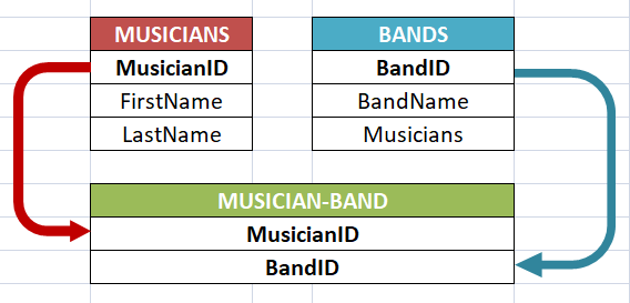
Red table contains musician information (MUSICIANS) and blue table contains band information (BANDS). A musician can belong to only one band, and in one band there can be one or more musicians.

The M:N relationship between MUSICIANS and BANDS has been dissolved into two one-to-many relations.

The 1:N relationship between MUSICIANS and MUSICIAN-BAND reads this way: for one instance of MUSICIANS there can be many instances of MUSICIAN-BAND; but for one instance of MUSICIAN-BAND, there exists only one instance of MUSICIANS. The linking table MUSICIAN-BAND has 2 fields, both are foreign keys, as they are primary keys in tables MUSICIANS and BANDS.

Core Excel functions for Data Analysis

Sunday, 26.06.2022

One of the common tasks in data analysis role is dealing with claims containing one or more products. If there is, for example, table of claims organized in the way that one record represents one product, there would be more than one records for the same claim, in case the particular claim contains more than one product. There is usually a field that contains particular product value, and once there has to be required to sum up values of all products within one claim. Of course, operation is simple and clear - just sum up values of the products that belong to the same claim. Request might look like this: add additional field (called calculated field) for each record, that would contain total claim value for each product. For such purpose it is used Excel SUMIF function, as shown in the table below:

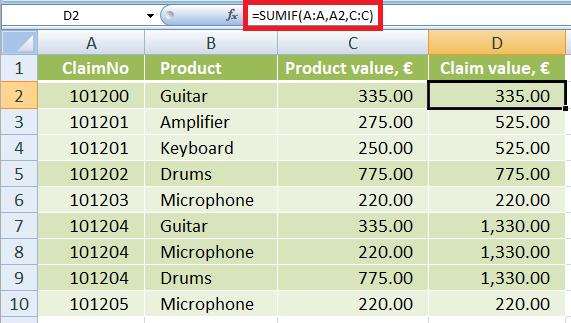
For the purpose of counting how many product there are within a particular claim, there is a COUNTIF function, that works similar as SUMIF function. The only difference is that COUNTIF actually counts number of lines that meet specified criteria - in this example lines that contain the same claim number, as shown in example below:

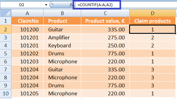
Both SUMIF and COUNTIF functions has options to specifiy more than one criterion, in that case it is to be used SUMIFS and COUNTIFS function. To calculate conditional average, maximum or minimum there are functions AVERAGEIF, MAXIF and MINIF, that work pretty much the same way as SUMIF, with slight difference in arguments order, as shown in further text.

AVERAGEIF(criteria_range, criteria, avg_range)
MAXIF(max_range, criteria_range, criteria)
MINIF(min_range, criteria_range, criteria)

Application of these functions in the claim model is shown in the following table:

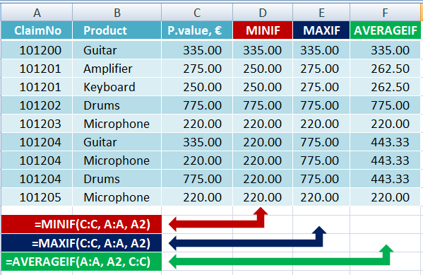
These functions have also their counterpart functions for specifing more than one criterion - AVERAGEIFS, MAXIFS and MINIFS. However, MAXIF(S) and MINIF(S) functions were introduced since Office 2016, so it's neccessary to make sure that everybody who works on your file should have Office 2016 as they otherwise will get #NAME? errors.

Unlike SUMIF, COUNTIF and AVERAGEIF, functions MAXIF and MINIF were introduced in Excel since Office 2016

To count unique values in certain column, function UNIQUE(col) can be used. But this function is available since versions Microsoft 365 and Excel 2021, so there has been many Excel tables out there that had to use some other way to count unique values in a column. There are many ways to that, and the easiest one is by using MATCH function combined with row reference obtaining by ROW function.

Using MATCH function is the best way to count unique values in a column, and it works in all Excel versions. It takes a value from a particular row, searches for that value in its column, for uniqe value returns 1 and for all other duplicated values returns 0.

Let's look at the following example: There is a 1st column that contains customer claims and a 2nd column containing product that belongs to the particular claim. One claim can contain one or more products. If there is a claim with many products than in a second row claim number is repeated in the 1st column and another product in the 2nd column.

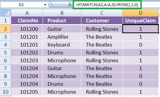
How could it be counted distinct number of claims? The way in actual version of Excel would be the by simply using UNIQUE function. But for backward compatibility and manage maintanance of existing tables created in previous Excel versions, MATCH function is the best option.

MATCH(lookup_value, lookup_array, match_mode)

Required argumets are lookup_value -value we are searching for, lookup_array - array where this value is being searched for, and optional argument is match_mode - 1 = exact or next smallest value (default), 0 = exact match, -1 = exact or next largest value. Return value is 1-based index of the row in which the value is found

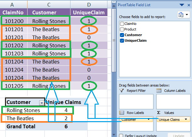
It is common practice to create a PIVOT table that contains only particular customers and that has to show number of claims for each selected customer. Using UniqueClaims claculated field created this way it can be accomplished in an easy and efficient way, as shown in the table above.

Data Analyst at 47 - to be or not to be?

Sunday, 29.05.2022

Is the age of 47 appropriate to be a Data Analyst? Is there a reasonable concern people in IT over thirty-five should have about their age to be a liability to their career? Well, some influential and respected trainers on Data Analysis field consider there are some more relevant factors than age(ism). Emotional maturity has become an appreciated trait, and it does not depend on age but on individual’s level of personal development.

High tolerance to frustration (as an element of the emotional maturity) is one of five soft skills that Alex The Analyst, who provides many excellent lessons on Data Analysis in his YouTube Channel, states as essential soft skills for the field:

self learning ability

having high tolerance to frustration

readiness for much manual work (with no automation)

capability to work with people

accepting not to get really reach

The ability to succeed in any role depends much more on one’s willingness to adapt, learn and unlearn, than on age.

Age brings experience

Nowadays - seven decades into the computer revolution, five decades since the invention of the microprocessor, and three decades into the rise of the modern Internet - it has to be taken into account that data science algorithms weren’t developed until the late 80's. Assuming you got in on the ground floor, the most experience anyone could possibly have as a data scientist is about 30 years. David A. Vogan Jr., the chairman of M.I.T.’s math department says experience matters in all sciences: “In a lot of the sciences, there’s a tremendous value that comes from experience and building up familiarity with thousands and thousands of complicated special cases.” How old is “too old” to be a data scientist? Assuming you have the skill set, there isn’t an age limit—even if you’re starting from scratch with a degree.

There is one evident fact regarding market demand on Data Analysts: it has been growing for years, and it is expected this trend will continue in the future. SalaryExpert has used average salary data gathered throughout the years to predict that the earning potential for data analysts entering the industry will increase by 21% over the next five years through to 2028

Back to the age topic. With years of experience, older applicants often bring far richer life and business experience. And this depth of knowledge can put them ahead of the younger competition. A recent study from 2021 by Zippia shows that average age of majority workforce in data analysis field falls into category over 40:

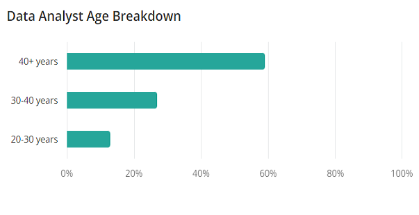
The common quality that all data analysts and data scientists possess, regardless of their age, academic or professional background, is strong quantitative skills. These strengths – often in math, statistics, and computer programming – are what make data analysts so valuable. Earning these skills is the most difficult part of becoming a data analyst. If you already have them, learning to leverage them in the data analysis process is a formidable but very achievable task.  If you have advanced qualifications, experience, or degree in a quantitative subject, you do not have to completely change career tracks to become a data analyst; you only have to learn a new way to apply your skills.

Traps of burnout & imposter syndrome

Among many potential traps that by experienced competitor is more expected to be avoided, there are two of most risky for the business: imposter syndrome and burnout. Someone might have imposter syndrome if they find themselves consistently experiencing self-doubt, even in areas where they typically excel. Imposter syndrome may feel like restlessness and nervousness, and it may manifest as negative self-talk. Symptoms of anxiety and depression often accompany imposter syndrome.

Burnout as commonly known and imposter syndrome (as maybe less known, but very common nevertheless) often come in combination, making a toxic couple that disables career development and leads to hell of helplessness, wrong conclusions and bad decisions.

Burnout is a reaction to prolonged or chronic job stress. It is characterized by three main dimensions: exhaustion, cynicism (less identification with the job), and feelings of reduced professional ability. More simply put, if someone feels exhausted, starts to hate their job, and begins to feel less capable at work, they are showing signs of burnout.

There are many advices out there about how to overcome those 2 dangerous threats, but the most important to even begin to address the problem is awareness what is going on. Both imposter syndrome and burnout have been among psychologists well known for years, and it's the matter of one's personal culture, knowledge and enlightenment to be able for problem to detect, accept and overcome. There are some of most recommended advices to overcome those 2 problems:

Be aware of the symptoms - knowing what imposter syndrome and burnout are and why it happens can help people spot the symptoms when they arise and apply strategies to overcome their doubts. Recognize a pattern in early phase.

Monitor your internal dialogue - ask yourself how you might support a friend who minimizes their accomplishments and then apply the same supportive language to your own narration

Talk about it - sharing feelings with or getting feedback from a trusted colleague, friend, or family member can help a person develop a more realistic perspective on their abilities and competence.

Challenge negative thoughts - swapping negative thoughts for positive ones is a key step toward overcoming imposter syndrome. Practice the following: celebrating current achievements, recalling past successes and keeping a record of positive feedback from others

Final thoughts

More experienced applicant has rich career behind themselves, often in more different positions. After working on many different roles, it is finished for them with the process of searching which role are they actually interested in, what they like and/or what they don't. They already know very well what they want and what they're good at. Choosing Data Analysis field after rich working experience is most probably a matture and adequate decision.

To make a long story short - age of 47 or any other is not an issue for the role of Data Analyst. Much more relevant factors are experience that brings potential to avoid traps such as burnout and imposter syndrome, tolerance to frustration, strong mathematical skills, flexibilty to adapt, ability to learn and - last but not least - deep personal interest, motivation and passion for the field.

Barry on Data Analysis-brief insights to relevant facts, definitions and best practices-

Data Analysis BLOG - description

Table of Contents

2022

2023

2024

2025

Full stack App deployment with containerization

NoSQL Database overview

JavaScript in Test Automation and beyond

JavaScript Intermediate (2)

Automated Test Containerization

JavaScript Intermediate

JavaScript Basics (2)

Playwright Test Automation with JavaScript (3)

Playwright Test Automation with JavaScript (2)

JavaScript Basics (1)

Playwright Test Automation with JavaScript (1)

Pytest & Playwright Web Automation Testing

Playwright basic features

Lambda functions and map()

Creating Pivot tables in Python

Exploring pandas Series

Is Data Analysis a Dying Career?

Specifying rules using CONSTRAINTs

R1C1 notation & German Z1S1 conversion map

Filtering, sorting & indexing data

Data connection modes in Power BI

Data Warehouse & Data Analysis

Database normalization - 1NF, 2NF and 3NF

Excel functions, tips & tricks

Reading files in pandas (csv, txt, json, xlsx)

Power BI basics

Using SQL for creating Pivot table

Python libraries - pandas

Data Analisys roles & goals

Branching, loops & functions

SQL essential features

LOOKUP function family

Built-in Data structures in Python

Database fundamentals

Core Excel functions for Data Analysis

Data Analyst at 47 - to be or not to be?

Playwright

JavaScript

Tips & tricks

Data Analysis

Excel

NoSQL

SQL

Python

Power BI

JSON

Statistics basics

Notes & Thoughts

Design Patterns

About the author

Who is this for?